EC 250 Macroeconomic Analysis
Course Takeaways
- What is the economy (i.e. output production. aka GDP)?
- goods and services created that can we can place monetary value on
- some activities may not be included like people staying at home instead of paying for daycare
- output is made up by capital stock, labour and a productivity factor, which doesn’t have numerical breakdown
- there are many ways to measure GDP
- goods and services created that can we can place monetary value on
- Without impacting consumption, only productivity determines long-run economic growth
- there are a variety of ways to improve productivity, read the section on policies long-run-growth policies
- Capital
- Capital are assets that people use to generate output
- Investments are made to maintain and grow capital
- Labour
- People choose to make trade-offs between leisure and money
- People want to fund their leisure time so work money for that purpose
- Obviously and unfortunately, there are situations where the person is living to work versus working to live
- Economic Cycle of busts and booms (“full employment”)
- “full employment” is where unemployment rate equals natural unemployment, something hard to measure and can change
- natural unemployment can exist due to matching issues (e.g. oil & gas jobs went to renewable sector) and due to the friction of changing jobs (hunting for a job after being laid off)
- Policies can be created to reduce matching issues and Employment Insurance can affect the friction (noticeable between provinces).
- shocks are what change the state of the economy drastically
- technology shocks (transistor, internet), productivity shocks (COVID-19), supply shocks (higher oil prices because of OPEC)
- Money
- exists for the sole purpose of making commerce efficient
- money can be interpreted as liquid assets meeting “what can be used to buy goods right now”
- money supply is influenced by the central bank and is made large because of fractional reserve lending
- for each dollar deposited at an institution, if the bank knows it only requires 20% to meet demand, it can lend until 80% has been fully lended (divide by 0.81)
- Inflation: increase in the price of goods and services
- can be deliberately induced by the central bank
- central bank policies have a lagging effect so money supply can grow in the past year and its effects may take another year
- goal of money supply growth is to reduce interest rates to spur investments
- money supply has no effects on full-employment in the long-term, short-term is up for debate since it does cause inflation
- if the money supply grows, market participants end up realizing their dollars are worth less in a real sense and will increase prices
- currently most central banks focus on annual inflation, but if they focused on stable price levels, then it would make it easier to properly invest today’s money. Inflation targeting results in $1 being equal to a range of values in 20 years rather than a single value, which would be the case if price level targeting was used instead.
- inducement by federal
- crowding out: interest rates go up (lower private investments) because federal government spending too much
- costs of inflation
- cost of updating price labels: shoe leather costs
- unanticipated inflation hurts savers and rewards banks and lenders
- hyperinflation: money loses meaning
- unexpected inflation and unemployment are related
- almost impossible to keep inflation unexpected
- can be deliberately induced by the central bank
Chapter 1 Introduction
Long-Run Economic Growth
- Developed countries have experienced extended periods of rapid economic growth whereas developing have either never experienced it or had periods of economic decline
- long-term growth: increase in output per unit of labour input (per worker, per hour) (aka average labour productivity)
- how to increase?
- 2016 Canadians 6x output than 1921 Canadians
Business Cycles
- short periods of slower and negative growth or rapid growth
Unemployment and Price Instability
- two key economic variables for measuring economic costs
- inflation: ongoing increase in prices of goods and services
- 1970s (10%)
- deflation: ongoing decrease in prices of goods and services
- Great depression (wages also fell)
- Policy makers guard against the threat of prolonged periods of deflation such as Japan has experienced since the 1990s (BUT WHY)
- Also don’t want to be like Zimbabwe with runaway inflation (hyperinflation)
International Economy
- open economy
- significant trading and financial relationships with other national economies
- closed economy: does not interact with rest of the world
- trading
- export: allows Canadian manufacturers to grow larger than if they were limited to the Canadian market
- import: allows Canadian consumers to choose from the best the world has to offer
- think: import fruits during Winter and export excess wheat
- When Exports > Imports, trade surplus.
- Trade deficit is when Exports < Imports.
- Exchange rate influences the trade balance
Macroeconomic Policy
- Fiscal
- Federal, Provincial, Municipal levels
- Spending
- Taxes
- Monetary
- Central bank
- Interest rate
Aggregation
- Aggregate consumption is the total consumer spending
- Not interested in finer details
- Interested in aggregate economic measures which is the sum of each variable
Macroeconomic Forecasting
- Forecasting is a small part
- long-term forecasting is too difficult as there are too many variables
- OPEC oil price
- Droughts
- Focus on interpretation of events as they occur (analysis)
- Focus on structure of the economy (research)
Macro Economic Analysis
-
Monitor the economy and figure out implications of current events
-
Private sector (impact on financial investments)
-
Public sector
- assist in policy making
- macroeconomic problems
- identifying and evaluating possible policy options
-
Actors: households, firms, and government
-
Change in income, interest rates, wealth influence on consumption
-
Motivations to increase/decrease taxes
-
Central bank responding to inflation
Economic Model Experiments
Evaluation of an economic model
- Are its assumptions reasonable and realistic?
- Is it understandable and manageable enough to be used in studying real problems?
- Does it have implications that can be tested by empirical analysis? That is, can its implications be evaluated by comparing them with data obtained in the real world?
- When the implications and the data are compared, are the implications of the theory consistent with the data?
Comparative Static Experiments
- Initial in equilibrium (demand = supply in all markets)
- A single independent variable is changed
- Events can be shocks (weather that affects wheat yields, discovery of new oil)
Disagreeing Macroeconomists
- always can find someone who disagrees with the status quo
- can even disagree with themselves
- positive analysis: economic consequences without desirability analysis
- what would happen if income tax increased by 5%
- normative analysis: whether a policy should be used
- should income tax be increased by 5%
Classicals vs Keynesians
- Adam Smith’s Invisible hand
- with free markets, individuals will do their own economic affairs for their interests resulting in the overall economy will working well
- Suggested wages and prices adjust fast
- issues; droughts, war, political instability
- developed vs developing
- argued that free markets makes people as economically well off as possible
- key assumptions: no minimum wage or interest rate ceilings
- classicists would argue for limited government role
- Keynesian
- Offered an explanation for the great depression’s high unemployment
- Suggested wages and prices adjust slowly
- Government should take actions to alleviate unemployment resulting in slow adjustment of wages and prices
- proposed solution: increase government purchases of goods and services
- demand for what resources?
- proposition was that to handle the demand, more people would need to be hired and then multiplier effect does the rest
- with what money?
Chapter 2 - The Measurement and Structure of the Canadian Economy
- measurement is possible and is required for serious understanding
National Income Accounting
The measurement of production, income, expenditure.
- national income accounts are an accounting framework used in measuring the current economic activity
- product approach: measure in terms of output produced (sold) excluding intermediate
- sum of value-added (output price - input costs)
- income approach: incomes received by the producers of output
- tax revenue, wages, after-tax profits (shareholder income?)
- expenditure approach: spending by the purchasers of output for consumption and not for input
- add up end user purchases
- total production = total income = total expenditure (fundamental identity of national income accounting)
Gross Domestic Product (GDP)
- broadest measure of aggregate economic activity
Product Approach
- Value-added = Output Sold - Intermediate Output + Inventory Increase
- some useful goods and services are not sold in formal markets
- homemaking, child rearing (and child breeding 😭) done by parents
- action to reduce pollution or otherwise improve environmental quality are not usually reflected in the GDP
- underground economy
- activity hidden from government
- illegal activity such as drug dealing, prostitution, etc.
- government services
- proposed to count at the cost to provide the service
- for housing markets, only new house sales are counted, realtor service is always counted though
- trucking/shipping is intermediary so isn’t counted…
- goods that are not used up, such as a lathe, are capital goods that are classified as final goods and included in GDP
- inventory increases are considered final goods because of “greater productive capacity”
- Gross National Product (GNP): domestic factors of production
- Canadian capital and labour used abroad
- net factor payments from abroad (NFP) is income paid to domestic factors of production by the domestic economy (GDP + NFP = GNP)
- GNP is crucial in countries where remittance is sent home (citizens working abroad)
Expenditure Approach
- income-expenditure identity
- Y = C + I + G + NX
- Y= GDP = total production = total income = total expenditure
- C =consumption
- domestic households on final goods and services (60%)
- durable goods (furniture, cars, appliances)
- semi-durable goods (clothing)
- non-durable goods (food and utility)
- services
- I = investment (25%)
- new capital capitals: fixed capital investment
- inventory investment
- government does make investments so that would go here
- G = government purchase of goods and services (20%)
- interest payments are not considered (good)
- is spending fueled by increase in debt counted? yes
- NX = net exports of goods and services
- Exports are spending done by foreigners (injection)
- Imports are spending done abroad
Income Approach
- Employee compensation
- Gross operating surplus (paid to owners of incorporated companies)
- do not include interest costs
- Gross mixed income (unincorporated enterprises)
- Taxes less subsidies on production (net taxes paid by corporations regarding production)
- Taxes less subsidies on products and imports (net taxes paid regarding the final output)
- statistical discrepancy
- expenditure approach minus income approach (added to income)
Private Disposable Income
- want to know how much income goes to private sector (households and businesses) so that demand for consumer goods can be predicted
- private disposable income = Y + NFP + TR + INT - T
- NFP = net factor payments from abroad
- TR = transfers received from the government
- INT = interest payments on the government’s debt
- T = taxes
- net government income = T - TR - INT
- GNP = Y + NFP
Saving and Wealth
- assets household owns minus what it owes = wealth
- national wealth is an important metric
- rate of saving
- national wealth depends on how much individuals, businesses, and governments save
Aggregate Saving
- Private saving = private disposable income - consumption = (Y + NFP + TR + INT - T) - C
- Private saving rate = Private Saving / Private Disposable income
- Government saving = net government income - government purchases = (T - TR - INT) - G
- budget surplus = T - (G + TR + INT)
- National Saving = private saving + government saving = Y + NFP - C - G
- Private saving is used for capital investment, financing for government, acquire assets from or lend to foreigners
- S = I + (NX + NFP) = I + CA
- Current Account Balance (CA) = NX + NFP
- payments received from abroad - payments sent abroad
- NFP is negative in Canada meaning foreigners earn more from ownership of Canadian factors of production than Canadians receive due to their ownership of foreign factors of production
- Private Saving = I - Government Deficit + CA
uses-of-saving identity. Private savings are used in three ways
- investment
- government budget deficit
- current account balance
Saving to Wealth
- Flow variables: measure per unit of time (e.g. annual GDP)
- Stock variables: one point in time (e.g. amount of money in your bank account on December 20th)
- flow is equal to the rate of change of the stock
- National Wealth = domestic physical assets + net foreign assets
- net foreign assets: foreign stocks, bonds, and factories owned by domestic residents minus foreign liabilities (domestic assets owned by foreigners)
- National wealth can change due to the values changing, or national saving dollar for dollar
- Therefore, national saving can be used to increase stock of domestic physical capital (I) and increase foreign assets
Nominal vs Real
- Nominal refers to current market values
- Does not work for different points in time since market values can increase due to inflation
- Real GDP, constant dollar GDP, measures GDP using prices of a base year
- Nominal GDP, current dollar GDP
- To convert, multiple outputs of GDP by price per output of the base year
Price Indexes
- Average level of prices for some specified set of goods and services
- GDP deflator: price index that measures overall level of G&S in GDP.
- real GDP = nominal GDP / GDP deflator
- Consumer Price Index
- Prices of consumer goods (basket)
- Concern is that the base year might get outdated due to changing consumer habits and goods available
- Inflation = (CPI_n / CPI_(n-1)) - 1
- Since 1989, inflation target for Canada is between 1 and 3% per year
- Can be overstated due to:
- quality/technology improvements
- substitutes
Interest Rates
- Rate of return promised by the borrower to a lender
- The nominal interest rate is the rate at which the nominal (or dollar) value of an asset increases over time.
- The real interest rate is the rate at which the purchasing power of an asset increases over time
- Varies according to who is borrowing, length, and other factors
- Real vs Nominal Rates
- real interest rate = nominal interest rate - inflation rate
- the nominal rate doesn’t account for that the nominal dollars might not buy more assets than the year before
- Expected real interest rate
- borrowers and lender act based on this
- r = i - expected inflation rate
- Expected inflation
- Difficult to determine expected rate
- Ask public
- Assume public has same expectations as what the government announces or private forecasts
- Extrapolate based on current inflation rates
Lesson 1 Summary
- Identify the major issues studied in macroeconomics.
- Explain what macroeconomists do.
- Highlight the similarities and differences between Classical and Keynesian macroeconomists.
- Discuss the three approaches to measuring national income.
- Identify key macroeconomic variables related to national income and discuss how they are related.
- Explain the meaning of these important macroeconomic statistics:
- Gross Domestic Product,
- Consumer Price Index,
- the inflation rate,
- the interest rate.
- Calculate the macroeconomic statistics (listed above).
- Discuss the distinction between real and nominal GDP.
- Calculate the GDP deflator.
- Explain the difference between real and nominal interest rates.
- Calculate the expected real rate of interest.
Chapter 3 - Productivity, Output, and Employment
- Labour market
- Goods and services market
- Asset market
- Full employment
- QS = QD
- Long-term behaviour
- Economic productive capacity
- The more an economy can produce, the more consumption, and the more saving and investing
- Quantities of input and productivity of the inputs
The Production Function
- If an economies factories, farms, and other businesses all shut down, other economic factors would not mean much
- Capital (factories, machines) and labour (workers, would autonomous AGI robots count?)
- Y = A F(K, N)
- Y = real output produced in the current period
- A = overall productivity (total factor productivity)
- K = capital stock, quantity of capital
- N = number of workers employed in the current period
- F = Function relating Y to capital K and N
- Cobb-Douglas production function: Y = A K^a N^(1-a)
- Under certain conditions, a corresponds to the share of income received by capital and labour gets 1 - a
Productivity and standard of living is highly correlated, but is it a casual relationship? I don’t think so. There has to be a common cause of both these two variables (obviously one being the income in the previous year, but I’d argue we need to look at monthly data since a year is simply the Earth traveling around the Sun but nothing really economical).
Canada Productivity
A = Y / (K^0.3 N ^0.7)
Statistics Canada: The Production Function of Canada 1981-2015
| Year | Real GDP Y (Billions of 2012 dollars) | Capital, K (Billions of 2012 dollars) | Labour, N (Millions of workers) | Total Factor Productivity A* | Growth in Total Factor Productivity (% change in A) |
|---|---|---|---|---|---|
| 1981 | 857 | 1019 | 11.3 | 19.66 | N/A |
| 1982 | 830 | 1048 | 10.9 | 19.30 | –1.8 |
| 1983 | 852 | 1063 | 11.0 | 19.63 | 1.7 |
| 1984 | 904 | 1078 | 11.3 | 20.37 | 3.8 |
| 1985 | 951 | 1100 | 11.7 | 20.86 | 2.4 |
| 1986 | 977 | 1116 | 12.0 | 20.89 | 0.2 |
| 1987 | 1022 | 1134 | 12.3 | 21.35 | 2.2 |
| 1988 | 1066 | 1165 | 12.7 | 21.61 | 1.2 |
| 1989 | 1091 | 1198 | 13.0 | 21.62 | 0.0 |
| 1990 | 1092 | 1225 | 13.1 | 21.37 | –1.1 |
| 1991 | 1070 | 1247 | 12.9 | 21.10 | –1.3 |
| 1992 | 1080 | 1253 | 12.7 | 21.40 | 1.5 |
| 1993 | 1106 | 1258 | 12.8 | 21.83 | 2.0 |
| 1994 | 1160 | 1273 | 13.1 | 22.48 | 3.0 |
| 1995 | 1190 | 1288 | 13.3 | 22.70 | 1.0 |
| 1996 | 1209 | 1303 | 13.4 | 22.83 | 0.6 |
| 1997 | 1264 | 1332 | 13.7 | 23.37 | 2.3 |
| 1998 | 1313 | 1362 | 14.0 | 23.70 | 1.4 |
| 1999 | 1386 | 1392 | 14.4 | 24.42 | 3.0 |
| 2000 | 1461 | 1424 | 14.8 | 25.14 | 3.0 |
| 2001 | 1483 | 1459 | 14.9 | 25.12 | –0.1 |
| 2002 | 1526 | 1483 | 15.3 | 25.31 | 0.7 |
| 2003 | 1555 | 1512 | 15.7 | 25.20 | –0.4 |
| 2004 | 1602 | 1553 | 15.9 | 25.47 | 1.1 |
| 2005 | 1654 | 1611 | 16.1 | 25.77 | 1.2 |
| 2006 | 1694 | 1678 | 16.4 | 25.77 | 0.0 |
| 2007 | 1732 | 1743 | 16.8 | 25.64 | –0.5 |
| 2008 | 1749 | 1810 | 17.0 | 25.36 | –1.1 |
| 2009 | 1694 | 1833 | 16.7 | 24.75 | –2.4 |
| 2010 | 1744 | 1887 | 17.0 | 25.01 | 1.0 |
| 2011 | 1798 | 1952 | 17.2 | 25.26 | 1.0 |
| 2012 | 1827 | 2024 | 17.4 | 25.17 | –0.4 |
| 2013 | 1871 | 2093 | 17.7 | 25.26 | 0.4 |
| 2014 | 1926 | 2165 | 17.8 | 25.63 | 1.4 |
| 2015 | 1938 | 2202 | 17.9 | 25.51 | –0.4 |
| 2016 | 1954 | 2212 | 18.1 | 25.56 | 0.2 |
| 2017 | 2022 | 2234 | 18.4 | 26.02 | 1.8 |
| 2018 | 2067 | 2258 | 18.7 | 26.28 | 1.0 |
- Marginal Product of Capital (MPK) is the additional units of output for every unit of capital. (delta Y / delta K)
- diminishing marginal productivity: MPK decreases as capital stock increases
- call centre where there is one telephone per cubicle vs there already being 5 per cubicle
- Marginal Product of Labour (MPN) is the additional units of output for every unit of labour. (delta Y / delta N)
- Supply/productivity shocks: a change in the production function
- changes in weather
- innovations or inventions in management techniques
- mini-computers, statistical analysis in quality control
- government regulations
- anti-pollution laws
- Ease and efficiency to access financial capital for facilitating day-to-day operations
Demand for Labour
- Since capital stock is long lived and investments only have a significant effect slowly, it is often fixed by economists when analyzing a few years
- year-to-year changes can often be traced to changes in employment
- assumptions
- workers are all alike (ignore aptitude, skills, ambition, etc. ) (why though? I feel that ambition & skills are very important, such as minimum wage jobs and non-minimum wage jobs)
- firms decide how many to employ, not at what wage to employ, that’s determined by competition
- firms hire based on maximizing profit (true but some company’s are hiring for growth and then doing mass layoffs)
- the benefit of the extra worker exceeds their cost
- when the marginal product of labour (MPN) equals the real wage (in units of output)
- Marginal Revenue Product of Labour (MRPN), measure extra revenue produced for adding another worker = Price times MPN
- MRPN = MPN * price = nominal wage
- We can also state that the real wage is determined by the output, so then we can state when MPN increases, increased employment / real wage increase
- the real wage is cost to employ (nominal wage) divided by selling price per unit
- The labour demand curve is relationship of the workers demanded and the real wage the firm faces (equal to MPN curve)
- N doesn’t have to be workers per se, could be hours
- It shifts due to supply shocks. Positive shocks increases MPN (and thus employment).
- Reducing payroll taxes would be a supply shock
- Reducing sales tax is not a supply shock. That’s a goods demanded shock
- Generally, an increase in capital stock also increases MPN
- Aggregate Labour Demand
- demand for labour of all firms in the economy
- Labour hoarding
- During a recession, hiring and firing costs are too much to otherwise layoff
Supply of Labour
- Each person decides whether to work or to do non-work actions (leisure)
- We want to give as many people possible the right to not work and not get paid
- A person who wants to make themselves as well off as possible, would work as much such that each hour worked makes up for each hour of free time given up
- Therefore, real wage = amount of real income that a worker receives in exchange for giving up a unit of leisure
- Substitution effect of a higher real wage: workers supply more labour in response to a higher reward
- Pure income effect
- when a worker’s wealth increases, the income is less valuable, therefore more time is spent on leisure
- when future wages will increase, there is an implied increase in wealth, therefore more time is spent on leisure
- long-term increase in real wage: both effects
- temporary no income effect since workers want to take advantage
- permanent we see income effect (aggregate supply of labour goes down)
- size of effect is dependent on each person’s situation include tax rates
- Suppose tax percent has increased just for the current year
- less likely to work since the time spent working is definitely less than letting go off leisure and since it’s only one year, the loss of income for one year isn’t convincing enough
- suppose there is a lump-sum tax (value not percentage)
- income effect only, so have to work more
- Labour Supply Curve
- quantity of labour supplied for the real wage
- shifts right if economy-wide real-wage rises
- Increase in wealth increases amount of leisure workers can afford (curve shifts left)
- Increases in expected future real wages increases amount of leisure workers can afford
- Increase in working age population increases number of workers (curve shifts right)
- An increase in the participation rate increases number of workers
- Equilibrium
- Classical model implies quick real wage adjustments
- Assumption is that people would be able to find jobs very quickly
- At equilibrium workers get a wage that just about equals the compensation for surrendering leisure
- When neither side is satisfied, something will have to give to get to Equilibrium
- When many workers are competing for few jobs, real wage falls
- full-employment level (N with line on top) at market-clearing real wage (w with line on top)
- have no accounted for unemployment yet
- A negative supply shock would decrease demand for labour (which equals MPN) at every level of employment so we could get lower wages
- there is a decrease in demand for labour because the expenditure for non-labour factors are higher and thus there is a lower optimal level
- Temporary, so labour supply curve does not shift
- Classical model implies quick real wage adjustments
Since more firms in Canada use petroleum as an input in the production process than produce oil as an output, increases in energy prices have generally been viewed as an adverse supply shock for the Canadian economy as a whole. Canadian firms have become more energy efficient due to these shocks.
Labour Market Equilibrium
- People earning under 40,000 (2011 dollars) have been the same since the 1980s, but the middle class is becoming richer
- Explanation is that there is unskilled labour and skilled labour, with the latter being the reason for the difference in wage increases
- Skilled-biased technological change occurs
- Full Employment Output (Y with line on top) = A F(K, N (with line on top))
- Education levels do not affect the labour market since the students are not part of the workforce and thus MPN has not actually increased (yet?)
- Things like energy supplies are other factors of production that can definitely impact the labour market (higher costs means higher MPN required)
- Immigration does increase output at full-employment, but of course real wages decrease due to the labour supply curve shifting right
- When skilled immigration increases, the real wages of skilled workers falls
- When unskilled immigration increases, the real wages of unskilled workers falls
Example 1
- Y = 9 K^0.5 N^0.5
- MPN = 4.5 K^0.5 / N^0.5 [derivative of above]
- NS = 110 * ((1 - t)w)^2
- K = 25
- Suppose t = 0 or t = 0.3. What is the equilibrium real wage and the level of employment?
- At full-employment, MPN = real wage.
Solution
1. w = 4.5 * 5 / (110 * ((1 - 0)w)^2) ^0.5
    w = 22.5 / (110w^2)^0.5
    w = 22.5 / 110^0.5 w
    w^2 = 22.5 / 110^0.5
    w = (22.5 / 110^0.5) ^0.5
    w = 1.4647
    N = 235.98

2. w = 4.5 * 5 / (110 * ((1 - 0.3)w)^2) ^0.5
    w = 22.5 / (110 * 0.7^2 w^2) ^0.5
    w = 22.5 / (110 * 0.7^2)^0.5 w
    w = (22.5 / (110 * 0.7^2)^0.5)^0.5
    w = 1.75
    N = 165.1
Example 2
- MPN = 400 - 4N
- NS = 18 + 10w + 2T (where T = lump-tax of 38)
- What is the equilibrium real wage and the level of employment?
Solution
Assuming MPN = w,
N = 18 + 10 (400 - 4N) + 2*38
N = 18 + 4000 - 40N + 76
41N = 4094
N = 99.85
w = 400 - 4 * 99.85
w = 0.60
3.5 Unemployment
- Not everyone who would like to work can find a job
- 54,000 households are surveyed every month
-
- Employed (worked full-time or part-time the past week or was on leave/strike)
-
- Unemployed (person was without work during the past week, sought a job in the past four weeks, and was available for work)
-
- Not in labour force (did not work and did not look for a job in the past four weeks)
- Employment-ratio is employed / working-age population
- Participation rate is the labour force / working-age population
- Discouraged workers: people who stop searching due to lack of success
- Unemployment spell: period of time an individual is continuously unemployed and the length of time is called duration
- Out of the unemployed, most have long durations, but most people who become unemployed have short-durations (low amount of workers with high churn compared to amount of workers with low churn)
- Reasons for unemployment
- Frictional: searching for suitable jobs
- Structural: chronic unemployment
- low-skilled workers are often unable to obtain desirable or long-term jobs
- could be because of inadequate education
- reallocation of labour from shrinking to growing industries
- low-skilled workers are often unable to obtain desirable or long-term jobs
- Natural rate of unemployment is the prevailing unemployment rate when output & employment is at full-employment levels
- Cyclical unemployment is the difference between the actual and natural unemployment rate (u vs u with overbar)
- My guess is that Canada’s natural rate of unemployment is between 5.5% - 5.6% because it was around this in 2019 and was below this during the inflation that occurred during 2022. When rates started going up, so did unemployment and now we are at 5.8% which I believe is still above natural unemployment due to the higher numbers of international students and the hours they can work.
Lesson 2 Summary
- Explain how output is determined using the production function.
- Sketch the relationship between output and capital (holding labour constant) and output and labour (holding capital constant).
- Discuss and calculate the marginal productivity of capital and labour.
- Analyze the impact of positive and negative supply shocks on the production function and output.
- Discuss the determinants of labour demand and supply.
- Discuss equilibrium in the classical model of the labour market.
- Discuss the categories of employment.
- Calculate key labour force variables.
- Discuss the different types of unemployment.
Chapter 4 - Consumption, Saving, and Investment
- Goods market equilibrium is when desired savings = desired investment
- Income (after-tax) = Saving + Consumption
- Desired consumption Cd
- Desired national saving, Sd occurs when Cd is met (in a closed economy)
- Sd = Y - Cd - G
Individual Consumption Decisions
- $20,000 income after taxes
- Could spend all of it or save some of it
- The future expectation may influence spending decisions today
- Could borrow to spend more this year, but the cost is bourne in the future
- Real interest rate r affects the trade-off
- Desire to have relatively even spending pattern over time is known as consumption-smoothing motive
def f(income_1=35_000, income_2=30_000, tuition=6150, i=0.05, wealth=0):
  desired_consumption = (wealth * (i + 1) + income_1 * (i + 1) + income_2 - tuition) / (2+i)
  print(f'desired consumption = {desired_consumption:.0f}, desired saving = {(income_1 - desired_consumption):.0f}')
  return desired_consumption, income_1 - desired_consumption
Current Income and Consumption
- Suppose $3,000 bonus after taxes
- Marginal propensity to consume (MPC)
- Fraction of additional current income that would be consumed in the current period
- When income reduces, it gives the fraction of current income lost that is saved
- If MPC is 0.4, and income lowered bt $4,000, consumption would reduce by $1,600
Expected Future Income and Consumption
- If income is expected to start coming in, consumption will be higher than if no employment opportunity was upcoming
Wealth and Consumption
- Similar the current income expect that expenditures clearly come out of savings and not out of the additional current income
- Because people own a part of their wealth in equities, the performance of the stock market ought to influence consumption spending
- Another major form of wealth is housing
- Therefore, one could argue, inflation could be cooled by decimating the housing market. If people who bought houses for investments get wrecked, they will spend more and thus prices will cool
- “5.7 cents for every dollar increase in housing wealth, but not measurable for increases in stock market wealth” - Lise Pichette, “Are Wealth Effects Important for Canada?,” Bank of Canada Review, Spring 2004.
- one third of households own stocks, two thirds own a house
- stock prices are more volatile
- primary household capital gains tax exemption
- concerns of a housing bubble that may one day burst may impact the whole economy ($4,000 less spending per house)
Real Interest Rate and Consumption
- higher interest rate is two pronged
- one hand: take advantage of higher payoff
- substitution effect of the real interest rate on saving (save more and spend more in the future)
- other hand: need smaller amounts to achieve target
- income effect of the real interest rate on saving
- need to consider people are borrowers as well
- borrowers can consume less when they have to spend more on interest
- the effect on real interest rates and national saving is not very strong but a higher national savings is said to lower real interest rate
Comments
- cars don't last as long as houses and require financing (interests) - houses are 10x car prices and have amortization period of 20+ years so higher interest rates means paying more in interest + you need to pay maintenance - some people are - interest payments on student loans (not applicable anymore due to federal laws allowing tax deduction) - the situation where real interest rates rise seems like during periods of high inflation → less inflation so maybe people had to reduce consumption and the temporary higher real interest rates just allows for returning to normal spending habits - when real interest rates rise, what are expectations for the stock market? If they are the same, then why would people save more? how many people are actually saving? - https://www.thestar.com/business/majority-of-canadians-now-have-more-debt-than-savings-statcan-says-here-s-why-the/article_40e0159e-b6fc-11ee-aaed-839d0983b705.htmlTaxes and Interest Rates
if i is the nominal interest rate and t is the income tax rate,
(1 - i)t is the after-tax nominal rate
Expected after-tax real interest rate
pie is the expected inflation rate.
Target overnight rate is the key indicator of monetary policy. The overnight rate itself is what chartered banks make on short-term loans to one another. Where is the repo market and who has access to it?
- Reserve ratio:
- how much banks must keep as reserves which prevents the banks from loaning out
- the central bank pays interest on the reserves (interest on reserves) for banks to deposit into the central bank
- Discount rate: how much it costs to loan money from the central bank
- Open Market operations: central bank can purchase or sell government treasuries which is an opportunity cost for banks when they lend to each other
- This is basically subsidizing by the central bank
Fiscal Policy
- The assumption is that fiscal policy does not affect aggregate supply of goods and services and that aggregate output Y is given
- This assumption is everything wrong with the economy. It’s why we are where we are and not in the future already
- If governments derived policies that targeted aggregate supply of goods and services in a way that creates jobs and not in a way that competes with other businesses for the G&S it bid for, Canada would be more innovative. How is green technology going to give us all jobs?
- The textbook says this assumption is valid at full-employment (people who are chronically unemployed can be hired though) and that the policy won’t significantly affect capital stock or labour supply
- Affects Cd which is that $1 less in consuming is $1 more in national saving
- Government spending can come from higher taxes which means less consuming
- If governments have to borrow, that means taxpayers have to pay more taxes in the future…expected future incomes will fall, thus reduced consumption
- Any temporary increase in government spending will reduce desired national saving because the new amount saved will always be less than the amount G spent
- With tax cuts thrown in, “anything goes”
- Consumers are not going to be thinking about future tax increases, so either government spending goes down the same amount as tax cuts or desired consumer spending will increase and national saving will decrease. If government spending went down an equal amount, then there would be higher national saving because of course not all the income that was kept would be spent.
- Ricardian equivalence proposition: that tax cuts or increases do not affect consumption
Investment
- increase capacity to produce and earn profits in the future
- fluctuates sharply over the business cycle and can account for half or more of declines
- goes down because of expected future profits / demand. Will government spending increase prices or actually lead to the intended chain effect of increased investment
- seems like during recessions, governments should be investing heavily to get better equity in startups/innovation rather than give grants
- important in understanding long-run productive capacity
Determinants of Desired National Saving
| An Increase in… | Desired National Savings… | Reason |
|---|---|---|
| Current output | Rise | Part of the extra income is saved to provide for future consumption. |
| Expected future income | Fall | Anticipation of future income raises current desired consumption, lowering current desired saving. |
| Wealth | Fall | Some of the extra wealth is consumed, which reduces saving for given income. |
| Expected real interest rate, r | Probably rise | An increased return makes saving more attractive, probably outweighing the fact that less must be saved to reach a specific savings target |
Desired Capital Stock
- Amount of capital that would allow the firm to earn the largest expected profit
- MPKf is the expected future marginal product of capital which is the benefit from one unit of investment today
- Example
- $1,000 oven per cubic metre
- no operational costs (solar-powered)
- 10% depreciation (10% less efficient every year)
- borrowing rate is 8%
- This is a cost because for every $ invested with borrowed funds or retained funds, it could’ve been earning the interest rate too!
- Therefore, the user cost is $180 per cubic metre per year it should equal MPKf for maximizing profits
- profit maximization after considering taxes: (1 - tau)MPKf = uc
- divide both sides by 1- tau to get the “tax-adjusted user cost of capital”
- actual corporate taxes are on profit not revenues and investment is sometimes deductible
- depreciation allowances
- investment tax credit
- therefore use effective tax rate: what tax rate (tau), on revenue has the same effect as the actual tax code
q theory of investment
- James Tobin, Yale
- that stock prices influence capital investment
- if Tobin’s q > 1, profitable to acquire additional capital since value > cost
- if Tobin’s q < 1, not profitable
- Tobin’s q = V / pKK
- V: stock market value of firm, pKK is the replacement cost of the firm’s capital cost (Maintenance CAPEX?)
- Higher MPK → higher stock prices → higher q
- lower real interest rates → shift from investing in bonds to stocks → higher stock prices → higher q
- lower capital purchase price → lower denominator and higher q
Changes
- decrease in expected real interest rate, increases desired capital stock
- higher capital stock means higher profits meaning higher stock prices as well
- technological changes increase MPKf
Taxes
Effective tax rates on capital investment G7
| Country | 2005 | 2010 | 2015 |
|---|---|---|---|
| Canada | 38.8% | 19.9% | 20.0% |
| Germany | 33.8 | 24.3 | 23.8 |
| Italy | 32.5 | 27.2 | 8.3 |
| United States | 35.2 | 34.6 | 34.6 |
| United Kingdom | 29.7 | 28.7 | 22.9 |
| Japan | 45.8 | 45.8 | 42.1 |
Is Japan high post flattening of GDP or was it always high?
Two opposing forces: purchase or construction of new capital goods (gross investment)increases capital stock but capital stock does depreciate and wear out which reduces the capital stock. I feel that with software, tech debt does not actually wear until it becomes unbearable and unproductive to use and/or update. The difference between gross investment and depreciation is net investment.
net investment = gross investment - depreciation
Kt+t can be replaced with the desired capital (K*)
Realistically, the investment cannot be made immediately and might take years as in the case of skyscrapers and nuclear power plants.
Determinants of Desired Investment
| An increase in… | Causes Desired Investment to | Reason |
|---|---|---|
| Real interest rate, r | Fall | The user cost increases, which reduces desired capital stock. |
| Effective tax rate | Fall | The tax-adjusted user cost increases, which reduces desired capital stock. |
| Expected future MPK | Rise | The desired capital stock increases. |
Investment in Inventories and Housing
- Inventory investment = increase in inventory of unsold goods, unfinished goods, or raw materials
- the most volatile component of investment spending during business cycles
- Residential investment: construction of housing, (SFH, condos, apartments)
Why might inventory spending increase?
- add more variety (e.g., for cars) for shoppers to select from to avoid waiting for delivery
- The expected commission (keeping the same sales force) from the increase dictates the spending inventory level
- Cost of holding more inventory (cars): depreciation, financing for the higher inventory
Apartment investments:
- marginal product is the real value of rents (that can be collected) minus taxes and operating costs.
- the user costs = depreciation, wear and tear, and interest costs
- construction incentive: future marginal product is at least as great as its user cost
As for other types of capital, constructing an apartment building is profitable only if its expected future marginal product is at least as great as its user cost.
Goods Market Equilibrium
- what economics forces at play?
- real interest rate plays a big part
- equilibrium is when aggregate quantity of goods supplied equals aggregate quantity of goods demanded
- equilibrium is when Y = Cd + Id + G
- difference between income-expenditure identity is that there are two desired components, so actual output vs. desired may be different.
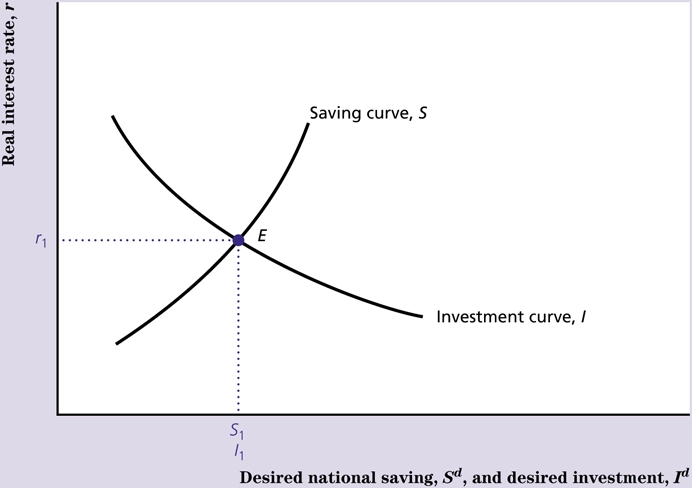
- Desired savings (Sd) = desired investment Id ; graph with interest rates being the vertical axis
- higher interest rates make investments more expensive as the competing rate of earning can be met in the bonds market or something
- There is some contradiction as now the text is claiming that higher real interest rates definitely increase national savings
- Apparently the real interest rate will be bid up. I guess because banks will have exhausted lending, so private credit lends at the equilibrium rate?
- The interest rate represents many rates so things get messy in real world
Shifts in the Savings Curve
- a temporary increase in government spending can result in savings curve shifting left (lower desired national savings)
- crowding out is when government spending (excess demand for resources) causes investment to decrease (due to the higher market-clearing interest rates)
- Apparently “expected increase in future income” does not shift the savings curve down
- net export crowding: if a fiscal expansion causes the local currency to appreciate, reducing the net exports.
Shifts in the Investment Curve
- new invention that increases MPK
- new economic reforms
Lesson 3 Summary
- Discuss the factors that underlie economy-wide demand for goods and services in a closed economy.
- Explain the determinants of household spending and saving.
- Explain the determinants of investment spending by firms.
- Describe how equilibrium is obtained in the goods market.
- Explain the role of the real interest rate in bringing goods market to equilibrium.
- Describe how equilibrium is obtained between saving and investment using the saving-investment diagram.
Chapter 7 - The Asset Market, Money, and Prices
Buy and sell financial assets such as gold, houses, stocks, and bonds
Money: assets that can be used to make payments, such as cash, and chequing accounts. Most prices are expressed in units of money.
What is Money?
- assets that are widely used and accepted as payment
- medium of exchange
- without money, bartering is done
- bartering flaw is that it is hard to find someone who has the item you have and is willing to trade it for what you have
- opportunity to specialize is greatly reduced
- without money, bartering is done
- unit of account
- uniform way to measure value of everything (naturally flowing from previous statement)
- not always the same as medium of exchange for countries with high and erratic inflation. WANT: currency stability
- store of value
- any asset could be a store of value
- money is held even with low return because it can be used as a medium of exchange
Measures of Money
- M1 + Monetary Aggregate
- Narrowly defined money
- Currency and Balances held in chequing accounts
- All of its components are accepted and used for payments
- 37.6M population so $2396/person
- does not include savings accounts
- M2
- M1+ plus somewhat less money-like comprise M2
- non-chequable deposits
- cheques cannot be written on these deposits
- Investment accounts
- M3
- GIC accounts (fixed deposits)
- non-personal term deposits
- FX deposits of residents (because they can be easily converted to usable currency)
The Money Supply
- amount of money in the economy
- partly determined by the central bank
- open-market operations
- open-market purchase: newly minted currency buys financial assets such as government bonds from the public
- open-market sale: sell government bonds to reduce money supply
- can also purchase bonds directly from the government (printing money)
- developing countries with low tax base
- racked by war or natural disaster (government spending is necessary to prevent loss of life, not the same as not welfare)
- BoC is treated as a private entity (independent) which is why national savings still decreases with government deficits
Portfolio Allocation
- which assets and how much of each asset to hold
- Expected Return
- the higher an asset’s expected return (after subtracting taxes and fees such as brokers’ commissions), the more desirable the asset is and the more of it holders of wealth will want to own
- Risk
- Uncertainty about the return an asset will earn
- Most people don’t like risk
- Liquidity
- A liquid asset can easily be disposed of if there is an emergency need for funds or if an unexpectedly good financial investment opportunity arises. Thus, everything else being equal, the more liquid an asset is, the more attractive it will be to holders of wealth.
- Time to Maturity
- amount of time until a financial security matures
- prefer shorter over longer
- expectations theory means average of short terms = long
- reality: longer = higher returns due to term premium
Types of Assets
-
Bonds
- Fixed-income securities
- Canadian bonds have very low risk of default. High liquidity
- Corporate bonds are higher risk and could be illiquid during troubling times -Stocks
- Corporate ownership
- Dividends
- Small businesses are owned by one or two people and its shares are not marketable
- Return is profits or selling the company
-
Houses
- Largest asset for most homeowners
- Benefit of shelter minus maintenance and property taxes
- Change in value of the land and the house
- Mistaken belief that there is no risk in holding wealth as housing. US Housing Crisis
- Very illiquid, could take months or years to sell BUT home equity line of credit (HELOC) is available
- Durable goods such as automobiles, furniture, and appliances
-
The demand for each asset is how much a holder of wealth allocated for it in their portfolio
-
US housing crisis: less regulation in the US led to 22% of all mortgages being sub-prime, combined with delayed interest rising resulted in delayed mass default (52% in Freddie Mac and Fannie Mae)
-
Mortgage Backed Securities containing these loans were sold to everyone even foreign investors meaning that that the collapse affected more than just the USA
Demand for Money
- Liquid and low return
- Factors:
- higher price level → proportional demand for more money
- 70 years ago, price levels was 1/10th meaning nominally, you’d need 10 times less money.
- higher real income → demand more money (real means implies more money)
- higher real income means more spending meaning more liquidity needed
- not proportional, as higher the income, more efficient investment (might require minimum balance)
- also lower the income, there might not just be as many attractive alternatives
- increase in interest rates on monetary assets compared to non-monetary assets → demand more money
- returns on alternative assets can sway the demand for money
- a decrease in interest rates for non-monetary assets increases demand for money
- higher price level → proportional demand for more money
- Other Factors
- Increase in Wealth, small increase in demand for money
- Higher risk in alternative assets increases demand for money. Money itself can be risky via erratic inflation.
- Liquidity in other assets will reduce demand for money
- Convertibility to cash (deregulation, competition, innovation in financial markets)
- Efficiency in payment tech will reduce demand for money
- Credit cards, ATMs, debit cards
- Md = aggregate demand for money, in nominal terms
- P = the price level
- Y = real income or output
- i = the nominal interest rate earned by alternative, non-monetary assets (e.g. bonds)
- L =a function relating money demand to real income and the nominal interest rate
- the interest on monetary assets is less volatile than the interest on non-monetary assets and is thus not statistically included
- Can also use r + pi^e to express in terms of real interest and expected inflation rate
Divide both sides by the price level to get the real demand for money. Also known as the money demand function
Elasticities of Money Demand
- income elasticity of money demand: increase in money demanded for 1% increase in real income. suggested to be 0.5
- interest elasticity of money demand: increase in money demanded for 1% increase in interest rates on non-monetary assets (NOT PERCENTAGE POINTS. THINK 0.10 to 0.101). suggested to be -0.3
- inflation decreases as demand for money increases
Velocity and Quantity Theory of Money
- Turn over of the money stock
- nominal GDP / nominal money stock
- real income / real money demand
- higher velocity means each dollar is being used in a greater dollar volume of transactions (assuming transaction volume is proportional to gdp)
- quantity theory of money: real money demand is proportional to real income Md / P =kY where k is a constant
- demand for M reduces velocity so innovations such as interest bearing chequing accounts can reduce the velocity
- M1 velocity has been declining over time
- M2 is long-term stable but not over short-term due to something like the stock market
- % Change in velocity = % Change in Real Income minus Inflation minus % Change in Money Supply
Asset Market Equilibrium
- each asset has a fixed-supply, so equilibrium is met when the quantity demanded for each asset equals the fixed supply
- linked to the price level
- Two groups: money (M = all assets that can be used for payments. assumed to pay im). non-monetary (NM) assets pay (expected real interest rate + expected inflation rate)
- Md (total money desired by everyone) + NMd (desired non-monetary assets) = aggregate nominal wealth (as in the sum of desired distribution of wealth = total aggregate wealth)
- M + NM = aggregate nominal wealth (wealth = the two components that make it up)
- Therefore, there is equilibrium when the quantity of money demanded equals the quantity of money supplied
- The nominal money supply M is determined by the central bank through its open-market operations
- any imbalance between desired national saving and desired national investment is bridged by foreign borrowing or foreign lending
- Price factor is nominal money divided by the real demand for money
- Under classic model, government spending increases price levels which means that output does not increase
- If the expected inflation rate decreases, there is lower demand for non-monetary assets (due to lower nominal rates) and thus a higher demand for money
Money Growth and Inflation
The growth in price levels (inflation) is closely linked to the growth in the nominal money supply.
- the rate of inflation equals the growth rate of the nominal money supply minus the growth rate of real money demand
With ηY (\eta_Y) being the income elasticity of money demand, then in the long run where nominal interest rates are constant, inflation can be stated as:
Suppose that nominal money supply growth is 10% per year, real income is growing by 3% per year, and the income elasticity of money demand is 2/3. Then, Eq. (7.12) predicts that the inflation rate will be 10% − (2/3)(3%), or 8% per year.
By subtracting the variable nominal yield on the real return bond from the fixed nominal yield on the conventional bond, the Bank can therefore obtain a measure of inflation expectations.
Learning Outcomes
- List the functions of money.
- Discuss the different measures of the money and how they relate to the money supply.
- Explain the factors affecting how people allocate their wealth among various assets.
- Discuss the key macroeconomic variables that affect money demand.
- List the variables in the nominal money demand function and explain the effects of changes in each variable.
- Explain how changes in the real interest rate and expected inflation affect nominal money demand.
- Describe how the real money demand equation is obtained.
- Explain how other factors affect money demand.
- Define and calculate elasticities of money demand.
- Explain velocity.
- Discuss the quantity theory of money.
- Describe how equilibrium is obtained in the asset market.
- Discuss how the money supply is related to the rate of inflation.
Chapter 5 - Saving and Investment in the Open Economy
- open economies mean countries can temporarily spend more than they produce (via imports)
- desired investment does not have to equal desired saving when foreign sector is involved
- When saving > investment, lend in international market (current account surplus). When saving < investment, international borrower (current account deficit)
- The current account indicates how much is available for net foreign lending
- It is essentially the net payments/income transferred from and to
Balance of Payments
- Current account has three separate components
- net exports of goods and services
- merchandise trade balance = merchandise exports - merchandise imports
- gets more attention in press than warranted
- services include tourism
- foreign students in canada are an export of services
- merchandise trade balance = merchandise exports - merchandise imports
- investment income from assets abroad
- interest payments, dividends, royalties (credit)
- payment of investment income is a debit
- NFP include this plus the wages & salaries of Canadians working abroad but it’s small enough to ignore…
- current transfers
- payments from one country to the other (e.g. foreign aid)
- current account balance
- add all credit items and subtract all debit items in the current account
- positive = current account surplus, negative = current account deficit
- net exports of goods and services
Capital Account = inflows - outflows
- When the capital account has a surplus, that means that the net foreign assets decrease because there was more inflows (purchases of domestic assets) than outflows (purchases of foreign assets)
- Transactions where the good being purchased was not currently produced won’t be included in the current account. Trade of existing assets is recorded in the capital and financial account. When domestic assets are sold to foreigners, it’s a financial inflow (credit) since funds are flowing into Canada.
Official Settlements Balance
- Official reserve assets (not domestic assets, foreign government securities, foreign bank deposits, IMF assets)
- balance of payments or official settlements balance is the net increase in a countries net holdings of reserve assets. Surplus when holdings increase and deficit when holding reduce.
Current Account Balance + Capital Account Balance = 0
- Reasoning: international transactions are swap of goods, services, or assets
- Suppose Canadian imports 75 CAD worth of goods from British exporter
- The exporter then purchases 75 CAD worth of pound sterlings from the FX market
- The purchase of the 75 CAD counts as a capital inflow (example is the central bank reducing its reserve currency)
- Not sure if FX Market counts as a capital inflow
- The purchase of the 75 CAD counts as a capital inflow (example is the central bank reducing its reserve currency)
- Statistical discrepancy when difference is non-zero
Net Foreign Assets and the Balance of Payments Accounts
- re-definition: net foreign assets: foreign stocks, bonds, and factories owned by domestic residents minus foreign liabilities (domestic assets owned by foreigners)
- changes: value of existing foreign assets and liabilities. acquisition of new foreign assets or liabilities
- net amount of acquisition is the current account surplus
- a deficit means selling of assets or acquiring more debt (net foreign borrowing)
If new capital bought with foreign debt is highly productive, the foreign debt would not be an economic burden.
Open Economy Goods Market Equilibrium
How to calculate savings: Investment plus current account (NX + NFP); CA = GDP - Investment - Consumption - Government
- In a closed-economy, CA = 0
- NFP determined by past investments so are not much affected by current macro-economic developments. Therefore, just look at net exports.
- Total spending by domestic residents is called absorption
- Y - National Saving?
Saving and Investment in a Small Open Economy
- a small economy cannot impact world real interest rate. Therefore the real interest rate is fixed
- a supply shock can cause savings to decrease and thus the current account surplus falls (if rates are low enough, then the current account deficit increases)
- a supply shock won’t impact investment since interest rates did not increase
- globalization
- Globalization in Canada: direct investment (influence management) vs. portfolio investment
Saving and Investment in Large Open Economies
- can affect real world interest rates
- domestic economy and foreign economy (rest of the world)
- the excess savings in the domestic market show up as the desired borrowing (foreign investment minus foreign saving) in the foreign economy
- the world real interest rate will be such that desired international lending by one country equals desired international borrowing by the other country
- The current account of the lender country rises (income receives from abroad)
- The sum of current accounts of all countries equals 0 (therefore, equilibrium is one big a system of linear equations)
Twin Deficits
- large government budget deficits and large current account deficits
- proposition: government deficit reduces desired national saving and thus reduces current account surplus (reduces capital outflows)
- A deficit due to higher government spending does reduce desired savings and thus also reduces the current account balance
- public savings decreases, so unless consumption decreases, national savings goes down
- A deficit due to tax cuts (meaning no reduction in spending) will increase consumption if the Ricardian equivalence does not hold
- The one thing to note is that in the long run, tax cuts without a reduction in government spending might end up hurting the national wealth as the interest paid by the government won’t be going to all Canadians
- Would require an increase in private saving, a decline in investment to offset, or a rise in current account deficit
- A decline in investment is unlikely as the government is either demanding more domestic goods or demand is maintained
- 100% saving is not possible due to the Marginal propensity to consume (MPC) which is ???
- A decline in investment is unlikely as the government is either demanding more domestic goods or demand is maintained
Chapter 8 - Business Cycles
What is a Business Cycle
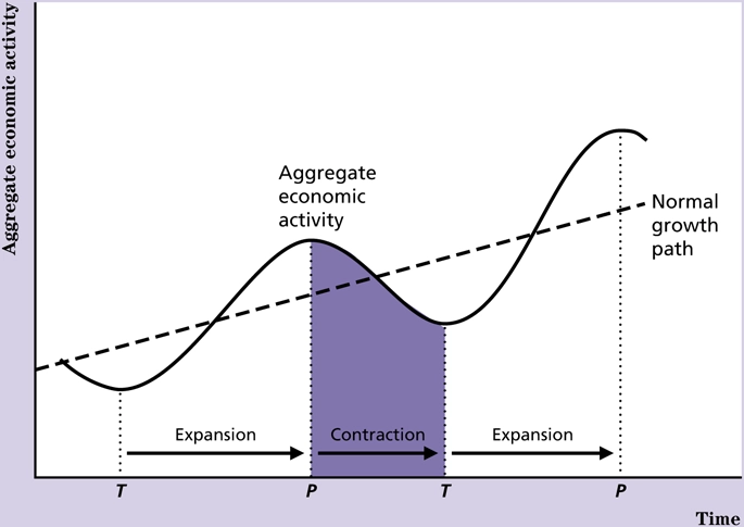
A trough is the low point in a business cycle and a peak is the high point.
A severe recession is called a depression. Sequence from one peak to the next is called the business cycle. Properties include:
- Fluctuations of aggregate economic activity
- Feature expansions and contractions
- Persistent
History shows that business cycles have become less severe, attributed somewhat to better monetary policies, but it could simply be better measurements, more job variability, or a lot of things. There’s no proof that all these factors will always be there, especially when some countries are not appealing to live in (e.g. UK).
Business cycles are periodic (bound to happen) but not known when to happen or the interval for it (not recurrent)
Economic Variables and the Business Cycle
economic variables can be:
- procyclical: moves with the business cycle
- countercyclical: moves against the business cycle
- acyclical: does not depend on business cycle
comovement: many economic variables having regular and predictable patterns over the business cycle
timing:
- leading: occurs ahead of of aggregate economic activity
- coincident: occurs at the same time
- lagging: occurs behind economic activity
Key variables
- production (procyclical and coincident)
- expenditure (procyclical and coincident)
- labour market variables (employment is procyclical and coincident; opposite for unemployment)
- money growth (procyclical and leads the business cycle)
- meaning: high money growth comes before business cycle expansion and lower money growth comes before contraction. Could also be counter-cyclical since Bank of Canada is trying to influence the economy
- CPI inflation is procyclical but lags
- financial variables (e.g. stock prices are procyclical and lead the business cycle)
- lead is like 1 month, so losses in stock market are followed by contractions?
- Durables vs. nondurables
- can put off purchases of durable goods when times are tough
- Output is more volatile than total hours
Explanation of Fluctuation
- economic shocks and models related to it
- classical or keynesian approach via AD-AS framework
Chapter 9 - IS-LM-FE Model
Full Equilibrium
- for the classical theory, full equilibrium (FE) condition which relaxes the Keynesian assumption of fixed wages in the labour market
- A situation in which all markets in an economy are simultaneously in equilibrium is called a general equilibrium
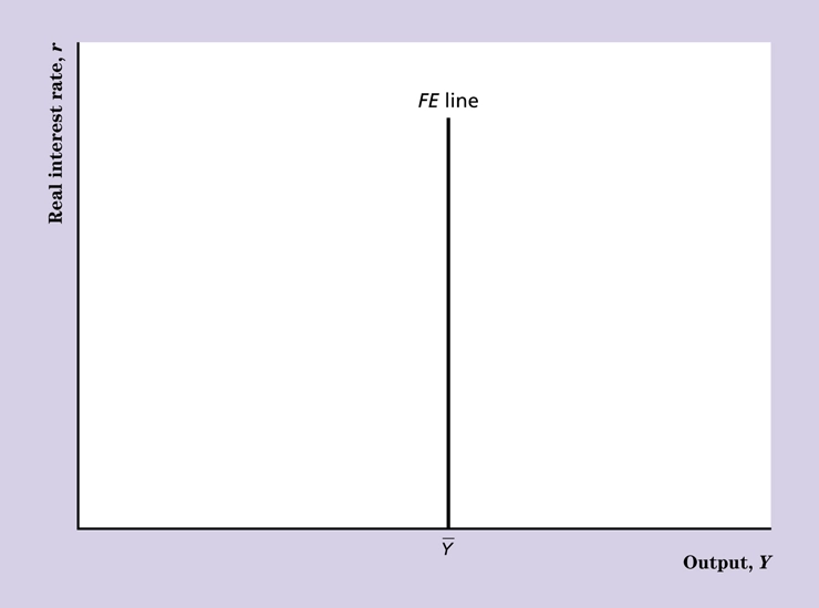
The full-employment line shifts right/left because of:
| All Else Equal, An | Shifts the FE line | Reason |
|---|---|---|
| Beneficial supply shock | Right | 1.More output can be produced for the same amount of capital and labour. 2. If the MPN rises, labour demand increases and raises employment. Full-employment output increases for both reasons. |
| Increase in labour supply | Right | Equilibrium employment rises, raising full-employment output. |
| Increase in the capital stock | Right | More output can be produced with the same amount of labour. In addition, increased capital may increase the MPN, which increases labour demand and equilibrium employment. |
Investment-Saving Curve
- Investment-Saving
- Savings and Investment equilibrium = goods market equilibrium
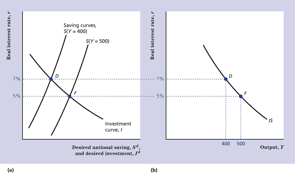
Factors That Shift the IS Curve
| All Else Equal, an Increase in | Shifts the IS Curve | Reason |
|---|---|---|
| Expected future output | Up and to the right | Desired consumption rises, raising the real interest rate that clears the goods market. |
| Wealth | Up and to the right | Desired saving falls (desired consumption rises), raising the real interest rate that clears the goods market. |
| Government purchases, G | Up and to the right | Desired saving falls (demand for goods rises), raising the real interest rate that clears the goods market. |
| Taxes, T | No change or down and to the left | No change, if consumers take into account an offsetting future tax cut and do not change consumption (Ricardian equivalence); down, if consumers do not take into account a future tax cut and reduce desired consumption, increasing desired national saving and lowering the real interest rate that clears the goods market. |
| Expected future marginal product of capital, MPKf | Up and to the right | Desired investment increases, raising the real interest rate that clears the goods market. |
| Effective tax rate on capital | Down and to the left | Desired investment falls, lowering the real interest rate that clears the goods market. |
Liquidity-Money Curve
- Price of non-monetary assets is inversely related to its nominal interest rate or yield
- For a given rate of inflation, the price of a non-monetary asset and its real interest rate are also inversely related
Basically, higher the price, lower the real interest rate. There is a different MD curve for each output Y.
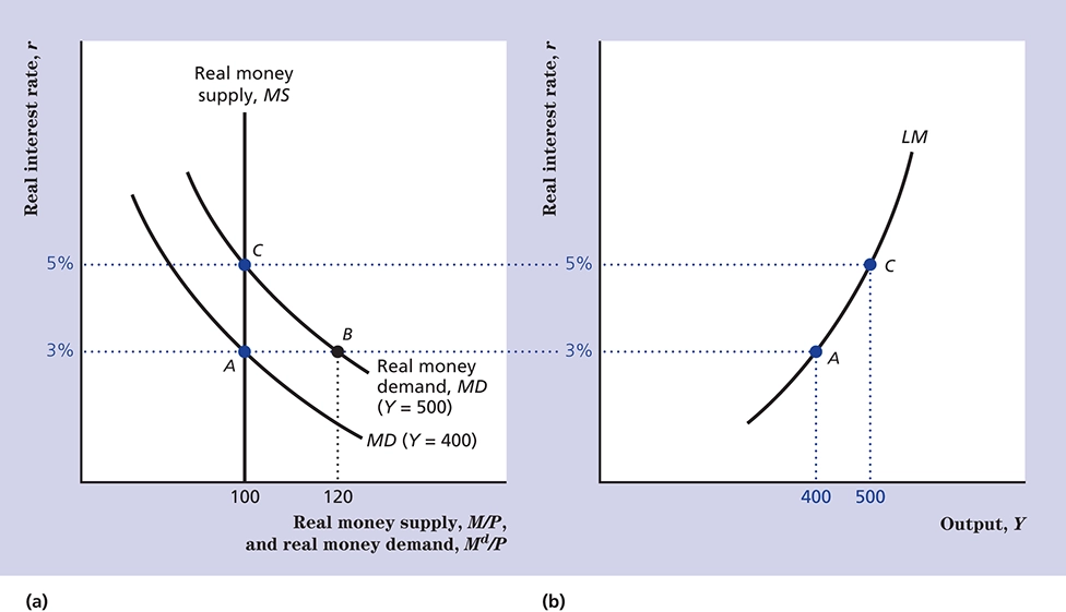
| All Else Equal, an Increase in | Shifts the LM Curve | Reason |
|---|---|---|
| Nominal money supply, M | Down-right | Real money supply increases, lowering the real interest rate |
| Price level, P | Up-left | Real money supply falls, raising real interest rate that clears the asset market |
| Expected inflation, pie | Down-right | Demand for money falls, lowering the real interest rate that clears the asset market |
| Nominal interest rate on money, im | Up-left | Demand for money increases, raising the real interest rate that clears the asset market |
Temporary Adverse Supply Shock
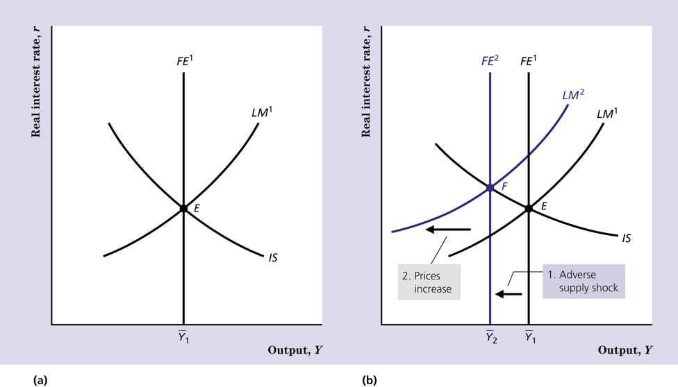
- Productivity falls temporarily,
- FE shifts left
- Price level adjust since IS and LS have a gap
- Real wage, employment, and output decline; real interest rate and price level at higher equilibrium point
- temporary inflation (higher price level)
- consumption and investment are lower
What is not consistent is that the real interest rate might not increase due to mismatched expectations; apparently if the shock is expected to be permanent, rates would not rise; the lesson says the shock was temporary, but historic oil prices shows that the oil prices stayed steady after 1974 till the next shock, whereas oil prices decreased after 1980. Real interest rates only rise if the expectation is that it is temporary.
1973-1974 Oil shock: USA gave $2.2B to Israel and OAPEC (OPEC Arab countries) decided to have an oil embargo on the USA. It is pretty clear that people would think this shock would be permanent. It’s not really clear why oil prices remained high even after the embargo ended in 1974. Prices most likely remained the same due to the devaluation of the USD by that time.
Constant: Government spending and nominal money supply
Monetary Expansion
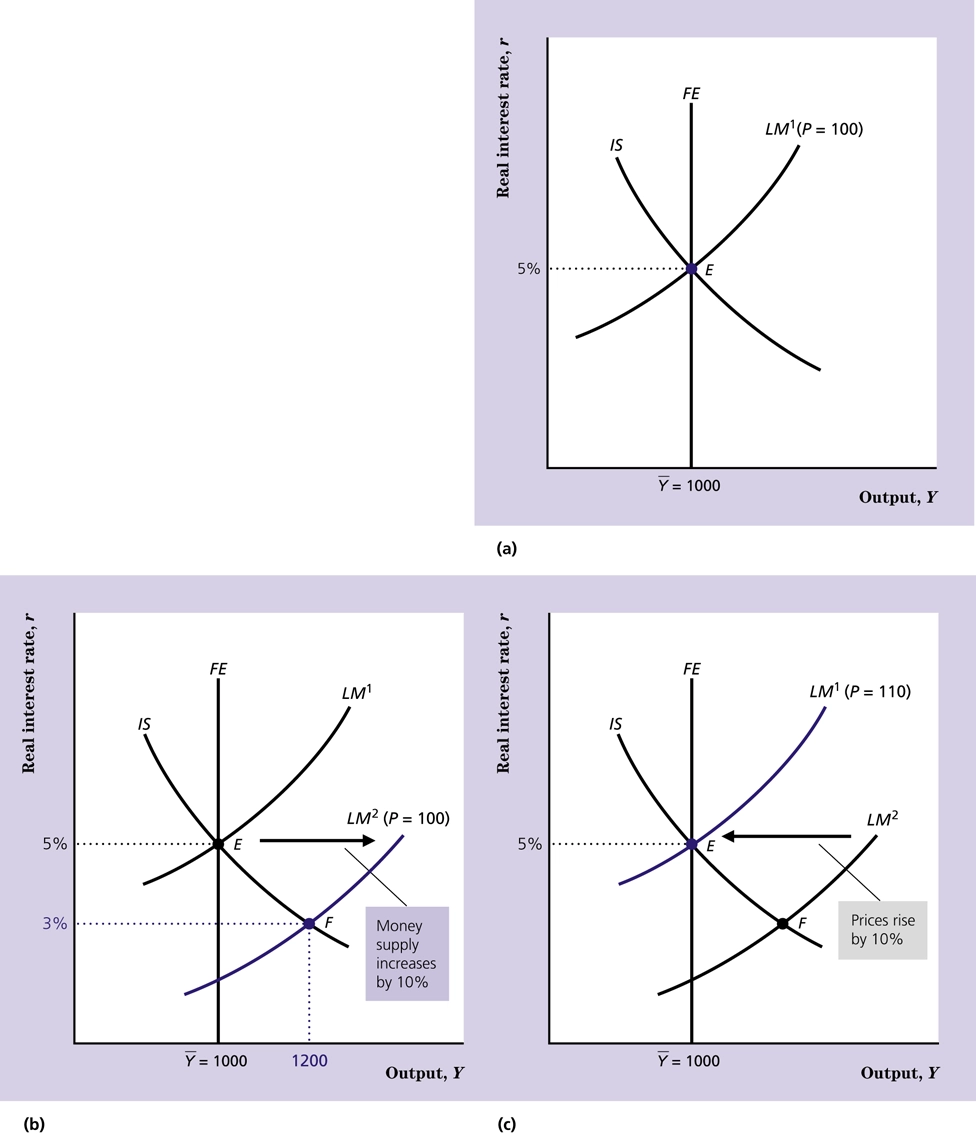
- short-term: lower interest rates and higher demand for output
- long-term: prices get higher but no net difference
Fiscal Expansion
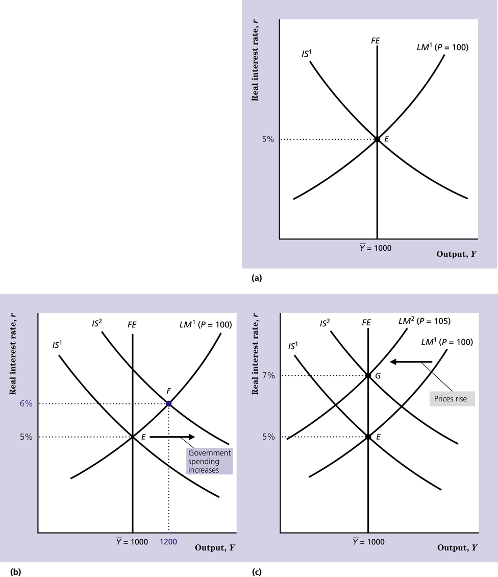
- government increases spending
- short-term: higher IS curve so higher interest rates
- long-term: prices and interest rates are higher
IS-LM-FE Classical vs Keynesian
- how rapidly is general equilibrium reached (could be 3 years in reality)
- what does monetary policy do?
- classical believes monetary neutrality exists in short-run whereas Keynesian only believes in long-run.
Aggregate Demand Curve
The relationship between price levels and output
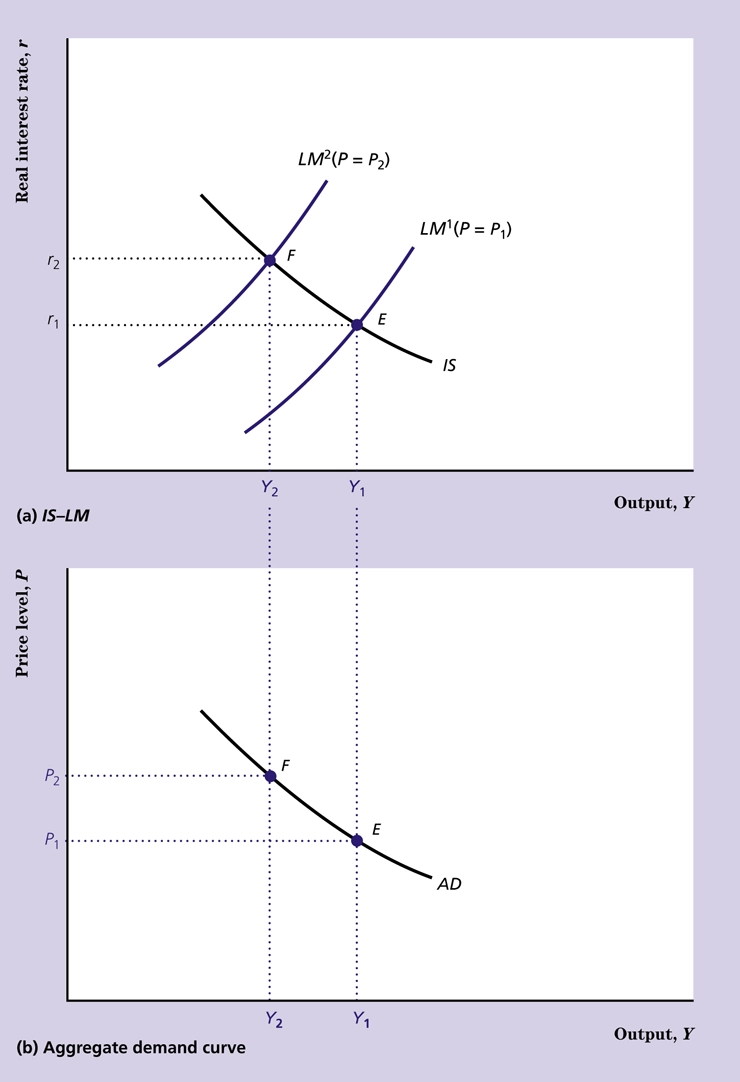
Factors that shift the curve is when the IS or LM shift while keeping the price level constant.
Chapter 9 Quiz Questions
Suppose the aggregate demand curve is given by the equation: Y =540 +30M/P.
The full-employment level of output is 1,500 and the current nominal money supply is 15. If the economy is in full-employment equilibrium, calculate the current price level.
P = enter your response here
With the price level fixed at 0.469, suppose the nominal money supply changes by 3 and is now 18.
Now find the short-run equilibrium level of output.
Y = enter your response here
To return to long-run equilibrium, the price level must adjust, shifting the short-run aggregate supply curve. The long-run equilibrium price level is:
P = enter your response here
Chapter 10 - Exchange Rates, Business Cycles, and Macroeconomic Policy in the Open Economy
Nation economies are interdependent in two main ways meaning policies of one country can affect the other
- International trade in goods and service
- Worldwide integration of financial markets
Nominal Exchange Rates
- Units of foreign currency that can be purchased with one unit of domestic currency.
- for most major currencies, enom is floating
- Canadian Effective Exchange Rate index (CEER) of 17 largest trading partners but moves in tandem with CA-US exchange rate
- Relative purchasing power parity: nominal rates change with inflation
Real Exchange Rates
- price of domestic goods relative to foreign goods such that
- if one hamburger in Japan costs 312 yen and one hamburger in Canada costs 3 dollars then the real exchange rate is 78 yen per Canadian dollar
Appreciation and Depreciation
- When the domestic currency appreciation: nominal exchange rate rises (buy more foreign currency)
- When the domestic currency nominal depreciation: nominal exchange rate falls (buy less foreign currency)
- fixed: weakening of the currency is called a devaluation while a strengthening is called a revaluation
Purchasing Power Parity
- holds in long run but not in the short run:
- countries produce different goods
- some goods aren’t traded
- transportation costs and legal barriers to trade
First factor is the appreciation and the last two factors are the inflation rates
Therefore, a nominal appreciation is either due to a real appreciation or a lower domestic inflation rate
Real Exchange Rate and Net Exports
This implies that the higher the real exchange rate, the lower a country’s net exports will be.
Demand for Currency
- able to buy goods from countries using said currency
- able to purchase real and financial assets denominated in said currency
Supply for Currency
- buy foreign goods
- buy foreign real and financial assets
Currency and Changes in Output (Income)
Rise in domestic output also meaning higher imports and lower net exports. Exchange rate decreases because they need to purchase foreign currency,
Effects of Change in Real Interest Rates
A rise in domestic interest rates makes foreigners want to buy domestic assets and strengthens the exchange rate
Returns on Domestic and Foreign Assets
Nominal rate of return on a foreign bond:
Interest Rate Parity
Suggests that there is an indifference between domestic and foreign assets of comparable risk and liquidity;
IS-LM-FE and Net Exports
- factors that increase net exports shift the IS curve up
- factors that decrease net exports shift the IS curve down
Factors that shift
- an increase in foreign output, which increases foreigners’ demand for domestic exports;
- an increase in the foreign real interest rate, which makes people want to buy foreign assets, causing the exchange rate to depreciate, which in turn causes net exports to rise;
- a shift in worldwide demand toward the domestic country’s goods, such as an increase in the relative quality of the domestic good
International Transmission of Business Cycles
- US output decline reduces demand for Canadian exports, shifting Canadian IS curve down
- therefore recession in Canada in a Keynesian model but in classical there is not affect
Mundell-Fleming Model
- small open economy IS-LM model which assumes that the exchange rate is not expected to change
- policies won’t affect foreign interest rates
Fiscal Expansion and Interest Rates
A rise in government purchases shifts the IS curve up and the domestic interest rate temporarily rises which induces capital inflows, appreciating the domestic currency, and thus making expert more expensive, such that IS curve shifts left until the domestic interest rate equals the foreign rate.
Monetary Expansion and Interest Rates
An increase in domestic money supply shifts the LM down, causing the domestic interest rate to fall below the foreign rate. Arbitrage opportunities induce capital flow into foreign from domestic, depreciating the domestic currency. A depreciated currency makes net exports cheaper, shifting the IS curve to teh right. The end result, assuming a fixed price-level, is an equal interest rate, depreciated currency, and higher net exports.
In the long-run, keynesian model shows monetary neutrality which occurs immediately for the Classic model; real exchange rate unaffected but nominal exchange rate is affected.
Fixed Exchange Rates
The nominal exchange rate is official set by the government, possibly in agreement with other countries. If the fundamental rate, determined by free market participants is less than the official rate, then the currency is overvalued. Responses include:
- The country can devalue the currency (by reducing the exchange rate) but if it did this a lot, it might as well employ a flexible-rate system.
- The country could also restrict international transactions to reduce the supply of its currency to the foreign exchange market, thus raising the fundamental value; even though this is suppression.
- Country could purchase its own currency via the central banks official reserve assets (gold, foreign bank deposits, and special assets created by agencies like the IMF). Reserve assets = balance of payments deficit. This method has its limits since some countries ran out of gold and thus a currency devaluation was inevitable.
- Similarly, an undervalued currency can’t be maintained for long by foreign central banks
- An undervalued currency can also be responded to by increasing the money supply
Monetary Policy and Fixed Exchange Rate
Countries have to co-operate with their monetary policies in order to avoid depreciating their currencies to another. If one country increases their money supply, the currency depreciates.
Fiscal Policy and Fixed Exchange Rate
- fiscal expansion results in undervalued exchange rate so the real exchange rate increases in lock step even though output is not impacted
Choosing an Exchange System
- a fixed exchange rate to promote trade,
- free international movements of capital, and
- autonomy over domestic monetary policy.
Currency Unions: Common currency shared by a group of countries (e.g. EU). Reduces cost of trading and prevents speculation attacks. Monetary policies cannot be independent.
Advanced Models of Open Economy
- the FE line to respond to unexpected events such as changes in world energy prices,
- expectations of exchange rate changes, and
- partial price level adjustment in the short run.
Quiz Question
- Why don’t PPP hold for Big Macs across the world?
- a. not exact productA
- b. sold by different franchises
- c. patent
- Nominal exchange rates of different trading partners is called?
- effective exchange rate
- If the dollar/Swiss frac exchange rate falls, then?
- dollar more valuable?
- swiss imports more from Canada into Switzerland
- canadian firms export more to switzerland
- swiss franc more valuable relative to the dollar
- 2002-2008 canadian dollar against US dollar appreciated due to net exports increasing
- If foreign interest rates decrease, then exchange rates rise and net exports decrease
- If Canada’s real interest rate rises relative to British real interest, we expect net exports to decrease but exchange rates to rise
- Increase is domestic income decreases net exports, increase in foreign income increases net exports. An increase in the domestic real interest rate results in a higher real exchange rate and a net exports decline
- In the short run in the Keynesian model for a small open economy with flexible exchange rates, an increase in the domestic money supply would cause domestic output to rise and the domestic real interest rate to fall
- for an undervalued currency in a fixed exchange rate, the country can increase money supply; if money supply is increased too much it may make the currency over-valued
- european union agreeing to use the euro is called a currency union. all countries in the currency union must share a common monetary policy.
Chapter 11 - Classical Business Cycle Analysis: Market-Clearing Macroeconomics
business cycle theories have two components:
- Description of the types of shocks believed to affect the economy the most
- a model that describes how key macroeconomic variables respond to economic shocks
Real Business Cycle Theory
Suggests that real shocks to the economy are the primary cause of business cycles; Real shocks affect the IS curve or the FE line while nominal shocks are shocks to money supply or demand which affect the LM curve. Examples of shocks:
- the production function,
- the size of the labour force,
- the real quantity of government purchases, and
- the spending and saving decisions of consumers.
The important shock is supply/productivity shocks.
Most economic booms result from beneficial productivity shocks; while most recessions are caused by adverse productivity shocks.
Critiques of RBC Theory
- cumulative effects
- other shocks such as war and military buildup
- counterargument: accumulation of smaller productivity shocks
Solow Residual
The proportion of growth not attributed to labour and capital
If there is a difference in intensity of inputs, productivity can change without technology changing. If uk is capital utilization, un is labour utilization, and A is tech,
Fiscal Policy Shocks in the Classical Model
An increase/decrease in government spending has a wealth effect (higher future taxes means poorer and income effects leads to more labour supply) that results in an increase/decrease in labour supplied shifting the FE line to the right/left resulting in an increase/decrease in the full employment level of output. Classic economists are against dampening the business cycle through fiscal policies.
Unemployment in Classical Models
In the classical model unemployment is just mismatched workers and jobs. With shocks, there is an increase in the matching problem. IMF reported great deal of churning of jobs but it doesn’t explain all unemployment (e.g. temporary layoffs; timing). You’d think more help would be needed during recessions but they fall. Government can reduce regulations on business or reduce minimum wage instead of fiscal policy that does not improve the matching problem (I mean the government can always expand government jobs).
Money in the Classical Model
procyclical is explained by “reverse causation”; the change in money growth precedes changes in output does not mean that the money growth caused the output changes. Storm windows don’t cause winter to come, the winter coming causes storm windows to be put up.
Bank of Canada wants to increase the demand for money by reducing the interest rate which requires a higher money supply so that businesses can get money they want easily and handle future sales. For example, just before christmas the money supply increases (gift-buying).
Misperception Theory; Non-Neutrality of Money
A producer’s wage is equal to the price of the good being produced. Price and output is related (higher the price more goods are produced and vice versa). The producer has to use previous expectations of the current price level to estimate the actual price level. So if there is an expectation of 5% inflation and price of bread increases by 5%, then baker retains output since the real wage has not changed. Therefore, the change in output can simply be due to the difference between the general and expected price levels.
We see here that supply can be higher if the actual price level is higher than the expected price level. This is because suppliers will think the a portion of the actual prices is real and will increase output to capture the difference.
So although Long-Run Aggregate Supply is vertical, Short Run Aggregate Supply is a curve swinging upwards intersecting when P = Pe. Anticipated monetary policy has no effects.
Rational Price Expectations Theory
If expectations are correct, the expected price will equal the actual price. The central bank has to surprise people to affect output but it’s clear that the central bank would want to increase money supply during recessions and decrease it during booms and so only a random policy would have effects.
Chapter 12 - Keynesian Business Cycle Analysis
- Non-Market-Clearing Macroeconomics
- Wages and prices are sticky and won’t easily go down
- Economy can be in disequilibrium for long period of time
- Recession is not an optimal response to an aggregate demand shock; rather it is disequilibrium in which high unemployment reflects excess supply of labour
- Stabilization policy can and should be used by the government to reduce economic fluctuations
Nominal Wage Rigidity
Nominal wages are set by contracts for an extended period of time and thus there are expectations of the future economy. Same equation as before. here is a different Short-Run Aggregate Supply (SRAS) for every expected price.
Monetary in the Keynesian Model
The IS-LM model is output versus interest rates whereas the AD-AS model is the Price level versus the output.
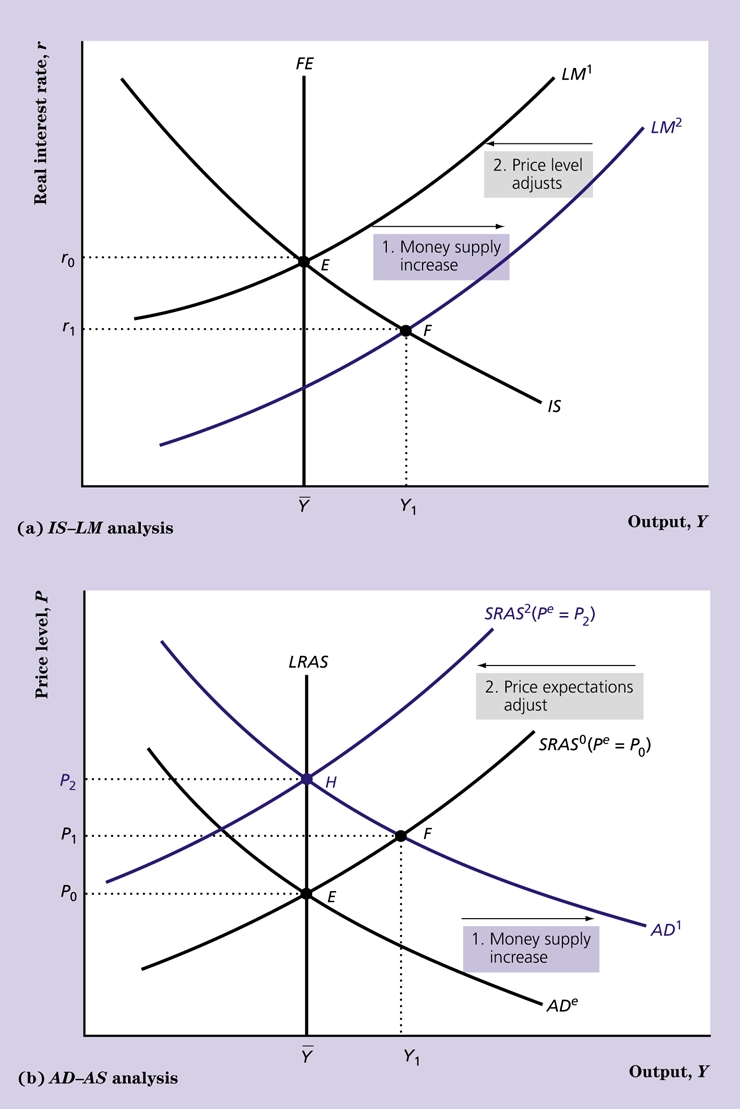
Fiscal Policies in the Keynesian Model
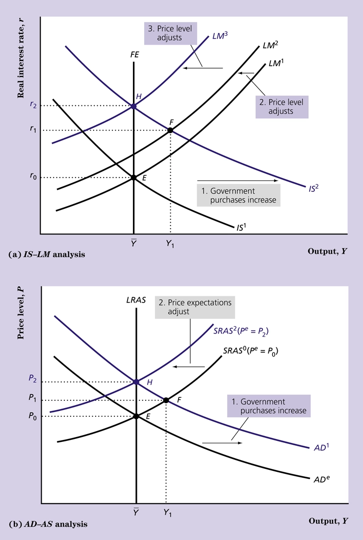
For an increase in money supply, there are two price level adjustments since one occurs before labour contracts are renegotiated
In the Classical model in the previous chapter, anticipated or unanticipated government spending influences wealth and the full employment output, whereas in the Keynesian model, participants anticipate the effects of the fiscal policy and negotiate a wage that would maintain the real wage (no change in wealth). With an unanticipated fiscal policy,
Fiscal and monetary policies are both referred to as aggregate demand policies because both policies affect the position of the aggregate demand curve. Only unanticipated fiscal policies have a long-term affect.
Criticisms of the Nominal Wage Rigidity Assumption
- less than one-third of the Canadian labour force is unionized and covered by long-term wage contracts
- some labour contracts are indexed to inflation, so the real wage is fixed, not the nominal wage
- real wages are procyclical no counter-cyclical
Price Stickiness
Empirical evidence on price stickiness is not conclusive; sticky in response to monetary policy shocks and flexible in response to shocks. Exchange rate pass-through is slow or incomplete.
- Monopolistic Competition
- Prices are set in nominal terms and maintain those prices for some period
- Output adjusted to meet demand at the nominal price
- Prices adjusted from due to significant changes in costs or demand
- Menu Costs
- Changing the price means printing new menus which costs money
For firms that have some monopoly power,
Price = (1 + Markup) * Marginal Cost
Macroeconomic Stabilization
Recessions are undesirable because the unemployed are hurt. Government policies can quickly restore to general equilibrium but would increase price level in the long-run tha if no action was taken. In my opinion, there shouldn’t be a need to fear people being unemployed if people could get a reduction in their tax bills equal to their estimated savings. Someone with $0 in savings should not have to pay as much in taxes nor should they get less in EI than someone who has $100,000 in savings. The latter can still maintain their assets so if anything EI should be as normalized as possible across the board. Secondly, there should not be a labour surplus during non-booming times. The government can also fund education during times of recessions so that people out of job can still get educated for skilled jobs that have labour shortages (grants given for specific programs).
Fiscal Policy Multiplier
- increase in gdp / increase in spending
- for the US economy the multiplier is sometimes zero during periods of full employment to 1.5 in periods of recession
- therefore, maybe best to run surpluses with full employment and deficits during recessions to avoid the price increase
Real Wage Rigidity and Efficiency Wage Model
- workers who feel well treated will work harder and more efficiently
- effort vs real wage is an S curve. There is a sweet spot just before effort flattens off (tangent to line from origin)
- therefore market-clearing wage > efficiency wage determines unemployment. Labour supply - Labour demand = unemployment and unemployment does not reduce real wages*
Demand Shocks
- more dispensable income (that is spent more than saved?) from a government tax cut or increase in money supply
- expected results -> higher output and prices immediately and then a return to full employment at a higher price level (SRAS curve moves)
Chapter 13 - Unemployment And Inflation
- Twin evils
- Phillips curve: an empirical relationship between inflation and unemployment
- inflation tends to be low when unemployment is high and high when unemployment is low
- only held till the 1960s as the relationship failed to hold in the decades that followed
- analysis to disprove the curve was also done during this time
- stagflation: where inflation and unemployment is high
- Expectations-Augmented Phillips Curve
- Friedman–Phelps theory
- Unanticipated inflation vs. cyclical unemployment
- In classical, Misperception theory is used
- When Aggregate Demand increases unexpectedly, cyclical unemployment will be negative because more employment than natural is required
- Example: think money supply is expected to increase by 10% (output remains equal), but increased by 15%. Price level increases less than 15% because output is increased as there is a belief that relative prices of goods are higher when they are not
- If unemployment rate is higher than natural, that implies that actual inflation is higher than expected inflation
- Strength of the relationship is related to the slope of the SRAS curve
Expectations-Augmented Phillips Curve
- When the expected inflation increases, the curve shifts to the right (higher unemployment rate for the same inflation rate)
- When the natural rate of unemployment increases, the curve shifts to the right
- For adverse supply shocks, classical blames the increase in natural unemployment to higher levels of mismatch between workers and jobs whereas keynesian blames it on higher than ideal real wage.
- classical: high energy costs transfers jobs from the energy users to energy providers (makes sense)
- Phillips curve moves up and to the right
- Beneficial supply shock leads to the curve moving down and left
Policies and the Phillips Curve
- Classical: stabilization policies are futile because of quick self-correction
- Keynesian: possible for unemployment rate to deviate from natural rate for an extended period of time
- Thus when AD falls and unemployment increases, government can use AD to increase inflation again
- The Lucas Critique
- new policies change the economic rules, and so no one can safely assume historical relationships will continue to hold
- applies to phillips curve when policy makers thought they could increase inflation to reduce unemployment
Long-Run Phillips Curve
- vertical line
- expected inflation = actual inflation
- actual unemployment = natural unemployment
Costs of Unemployment
- loss of output because fewer people are employed
- borne on the unemployed (loss of income) and society (unemployment insurance received instead of income taxes paid)
- Okun’s law: 1 percentage point increase in cyclical unemployment reduces real output by 2 percentage points.
- considered too high because it reflects more issues than just a change in cyclical unemployment
- offsetting factors:
- searching for the perfect match may lead to future productivity and output growth
- leisure time (diminishing utility)
Long-Term Behaviour of the Unemployment Rate
- natural unemployment rate corresponds to full-employment output
- unsure when we are at full-employment output
- hard to figure out what the natural rate is so not a good idea to pursue policies in pursuit of this number
- changes:
- Demographic
- women have equal or lower unemployment rate nowadays
- younger workers have higher unemployment rate
- Technological changes
- Higher skill requirement which reduces employment opportunities for low-skilled or poorly educated workers
- (see the Application “Technological Change and Wage Inequality” in Chapter 3, p. 74).
- Hysteresis
- the tendency of the natural rate of unemployment to change in response to the actual unemployment rate, rising if the actual unemployment rate is above the natural rate and falling if the actual unemployment rate is below the natural rate.
- downturns in economies with high levels of worker regulation tends to persist more due to firms not hiring workers that will never need to be fired (pessimist hiring versus optimistic)
- Employment Insurance
- replacement ratio: benefit relative to lost wages
- benefit duration: amount of time an unemployed worker receives benefits for
- eligibility requirements: what does the worker need to do to collect benefits
- disincentive index: disincentive to search for jobs and accept job offers
- Demographic
Policies to Reduce the Natural Rate of Unemployment
- no surefire method for reducing the natural rate exists
- make it easier for workers who have been made unemployed by a shrinking industry to retrain and find re-employment in expanding industries
- a case can be made for such policy measures as tax credits, subsidies for training, and relocating unemployed workers
- goal: eliminate mismatch between workers and jobs
- recent modifications of EI emphasizes retraining and encouraging workers to move to where new jobs are created
- minimizing size of payroll taxes firms pay when employing workers. Cost to employ includes contributions to EI, Worker’s Compensation, Federal and Provincial (Quebec) Pension Plans
- hysteresis proponents: aggressive monetary and fiscal policies (high pressure)
- not a good idea as it is high risk for a loosely validated problem of skill deterioration
There are definitely more policies that could be applied and more discussion should be applied in this area. For example, the textbook does not discuss information gaps between government organizations and individual workers, unemployed, and future workers. If innovation drivers economic growth, then shouldn’t worker’s be made aware of programs that they can contribute to. Or how to incentivize workers to become forefront of innovation (e.g. university grants in sectors that aren’t saturated).
Costs of Inflation
- Anticipated inflation:
- prices of goods and services would increase 4% every year, but so would nominal wages. No purchasing power harm
- nominal interest rates would adjust to offset drop in purchasing power; money saved would earn the real interest rate regardless of the rate of the anticipated inflation rate
- Shoe leather costs
- Costs incurred to reduce holding the cash whose value erodes due to inflation
- Estimated to be 0.3% of GDP for 10% perfectly anticipated inflation
- Menu costs
- cost of changing nominal prices; lowered by technological progress
- Unanticipated Inflation
- Interest earned in savings account is a less than expected in a real sense which is a gain for the Bank paying the interest
- lenders and savers get hurt, fixed rate borrowers or people with fixed payments benefit
- Hyperinflation
- extremely high for sustained period of time
- workers paid more often
- higher shoe leather costs
- the real value of taxes collected by the government falls sharply during hyperinflation
- when prices aren’t reliable indicators of supply and demand, then markets cannot allocate resource efficiently
Fighting Inflation
- sustained monetary growth in industrialized countries is usually due to not tightening monetary policies during times of over full-employment output but using expansionary policies during recessions
- disinflation by ways of slowing reducing the money growth may lead to a serious recession
- if policies succeed in reducing inflation below expected rate, unemployment will rise above the natural rate until inflation expectations lower
Rapid vs. Gradual Disinflation
Classical’s cold turkey
- rapid disinflation / reduction in money supply growth. Since it’s dramatic, public ought to reduce expectations
- Keynesian disagree because of an adjustment period which brings in delays and that people might expect the government to abandon the policy
Keynesian gradualism: reduce rate of money growth and inflation gradually over the years; effective due to being politically sustainable
The sacrifice ratio
- amount of output lost when the inflation rate is reduced by 1 percent
- Take the total output loss as a % of one year’s GDP, and divide it by the reduction in inflation
- different in every country, sometimes less than 1 and sometimes up to 3
- flexibility of the labour market. The higher the flexibility, the lower the sacrifice. The higher the regulation, the higher the sacrifice
- rapid disinflation tended to have lower sacrifice ratios
- Hard to determine if Laurence Ball’s estimate on the loss of output is accurate (e.g. supply shocks, estimating output without disinflation)
Credibility and Reputation
Saying is one thing and the electability of policymakers can get in the way of keeping promises. Central banks are usually independent.
Wage and Price Controls
- impose price and wages limits to break expectations
- price controls likely to cause shortages since in a free market, relative prices will change due to supply and demand
- shortages due to excess demand cause disruptions
- the disruptions imply that the controls are temporary and public will expect greater inflation in the future
- when combined with tightening, expectations of lower inflation post-lifting are more plausible
Chapter 14 - Monetary Policy and the Bank of Canada
Money supply is also affected by the banking system’s behaviour and the public’s decisions, not just the central bank.
- depository institutions: privately owned banks, trust companies, credit unions, and caisses populaires (Quebec) that accept deposits from and make loans directly to the public.
- First supply of money is deployed in exchange of real assets
- The belief that money has value becomes self-justifying: If most people believe that money has value, then it has value.
- if everyone believes money has no value then no one would accept it
- Convincing the public by declaring money as legal tender: creditors must accept the money as settlement of debts and can pay taxes in it
- Money is a liability on central banks’ balance sheet and it is the monetary base or high-powered money
Fractional Reserve Banking
- Money held as bank deposits instead of currency.
- bank reserves: liquid assets available for withdrawal and paying cheques drawn on depositor’ accounts
- 100% reserve: profit earned from negative interest rates (fee for deposit)
- partial reserve: not all currency is being used, some amount is being untouched. Therefore can lend it out to earn interest
- reserve-deposit ratio: reserves divided by deposit
- fractional reserve banking: reserve-deposit ratio is less than 100% (one)
- Since a loan ends up being deposited again, the bank will keep loaning out money
- Since the reserves amount never changes, the deposits will keep going up
- Therefore, the money supply balloons
- Money supply = monetary base / desired reserve ratio
Bank Runs
- when more depositors want to withdraw than the bank has money available
- from a depositors’ perspective, withdrawal avoided the risk of collapse
- banks would need to convince customers that everything is fine
Money Supply Formula
- M = CU (currency held by public) + Deposits
- BASE = CU + Reserves
- cu = Currency Deposit ratio (CU / DEP)
- res = RES / DEP
- M =((cu + 1) / (cu + res)) BASE
- The money supply equals the base times the money multiplier factor
Open Market Operations
- Central bank prints money and buys real assets with the money, thereby increasing the monetary base
- Central bank can also sell real assets and retire currency (lowers the currency and base)
- If the money multiplier is constant, the percent change in the monetary base equals the percent change in the money supply
- Since money multiplier is unstable, changes monetary base is used to influence short-term interest rates
Bank of Canada
- Created in 1934, crown corporation since 1938
- While the government may issue a directive to the Bank, it has not done so since the act was amended in 1967 to allow this
- Board: 12 part-time directors, governor (appointed for 7 years renewable by the governor), senior deputy governor, deputy minister of finance
- directors are not experts on monetary policy and cannot be bankers nor economists'
- Essentially, although the government has the power to influence the bank, it can’t influence in the short-term
- Balance sheet
- Largest asset are government bonds
- Owns nearly 20% of outstanding treasury bills
- Owns loans to other banks
- Notes in circulation (January 2023): 119,417,195,000
- Deposits from other banks plus currency at banks equals total reserves
- Monetary base = bank reserves plus currency outside banks
- Monetary base = total currency outstanding plus bank deposits
- Lender of last resort
Tool 1: Overnight Rates
- Banks only make net transfers to each other (e.g. National Bank $100 cheque from RBC + RBC $80 cheque from National Bank = $20 to NB)
- Clearing/Settlement balances are held at the Bank of Canada
- Reserves are not required to be held at the Bank of Canada, but 13 large banks and credit unions (direct clearers) do so.
- Large Value Transfer System (LVTS)
- Financial Institutions that can clear cheques but don’t partake in LVTS have accounts with the larger banks
- Banks with larger balances than needed can lend to another bank charging an overnight rate
- Bank of Canada announces on eight preset days (or in unusual circumstances) a 0.5 interest rate band of which the center is the target overnight rate
- The bank lends at the top range of the band called the bank rate which is a ceiling for the other banks
- The bank pays interest on deposits at the rate given by the bottom edge of the band which places a floor under the overnight rate
- Therefore, banks will only want to lend at a rate higher than this deposit paying rate and will want to borrow only at most the bank rate
- Lowering interest rate, increases advances made, which is a credit to deposits, which means the monetary base has expanded
Tool 2: Open-Market Operations
- Purchasing securities increases the bank’s assets and writes a cheque on itself (it’s own deposits)
- Multiplier effect results in a higher money supply
- Can be used to affect interest rates as well
- Special Purchase and Resale Agreements (SPRAs or repos): buy short-term government securities and sell next day (increase in seller’s settlement balance which puts downward pressure on the overnight interest rate)
- Sale and Repurchase Agreements (SRAs)
- Quantitative Easing
- Although most open-market operations are on short-term (3 month), it can buy/sell other things
- Purchase and sale of government or non-government securities with long terms to maturity
- once nominal interest rate reaches 0, bank cannot force it down any further, so QE can be used on the other assets
- Interest rates can be long-dated, illiquid, and risky so bank can either
- reduce rate of return on short-term, liquid, and safe to expect that others will move in same direction (conventional)
- reduce rate of long-term, illiquid, and risky by buying and selling those very securities (QE)
Tool 3: Exchange Fund Account
- various currencies (fraction of US dollars has fallen from 97% to just 69%)
- falling importance of gold (no gold held in 2020)
- reflects fund should yield a predictable rate of return
- Suppose interest rates rise in the US, bank of canada might want to start selling US dollars to counteract the depreciation passing as inflation
Monetary Policy in Practice
- lags and uncertainty about the channels through which monetary policy works
- 18 to 24 months to work their way through the economy to have significant effect on rate of inflation
- change in interest rate → change in spending → changes in production (employment) → changes in prices (inflation)
- interest rate channel: affecting the economy via real interest rate changes
- exchange rate channel: affecting the economy via real exchange rate changes
- credit channel: supply and demand of credit (changes in bank reserves)
Monetary Policy - Rules Versus Discretion
- Rules
- Monetary policy should be automatic
- e.g. 1% money supply growth every quarter
- e.g. keep price of gold stabilized (gold standard)
- must be simple
- Discretion
- the central bank should continuously monitor the economy and, using the advice of economic experts, should change the money supply as needed to best achieve its goals
Monetarist
- Dominant figure: Milton Friedman
Proposition 1. Monetary policy has powerful short-run effects on the real economy. In the longer run, however, changes in the money supply have their primary effect on the price level
Proposition 2. Despite the powerful short-run effect of money on the economy, there is little scope for using monetary policy actively to try to smooth business cycles.
- time needed to gather and process information (information lag) to determine state of economy
- uncertainty to the magnitude of the effect of a change in interest rates and money supply
- maybe a year to take effect
- bank of canada estimates 12-18 months to influence inflation rate
- might be possible for wages to adjust quick enough that the monetary supply causes prices to rise
Proposition 3. Even if there is some scope for using monetary policy to smooth business cycles, the central bank cannot be relied on to do so effectively.
- distrust of central bank comes from historic examples
- 1929-1933: Federal Reserve System was unable or unwilling to stop the money supply from falling by one-third due to bank runs
Proposition 4. The central bank should choose a specific monetary aggregate (such as M1 or M2) and commit itself to making that aggregate grow at a fixed percentage rate, year in and year out.
- central bank has considerable influence over the rate of money growth so it can be held accountable for deviation
- steady money growth would lead to smaller cyclical fluctuations than “countercyclical” monetary policies used historically
- ultimately, the growth rate of the monetary aggregate selected would be consistent with an inflation rate near zero
- some are open to suspending rules during a depression
Central Bank Credibility
Monetarism relies on the assumption that the government and the central bank are incompetent and can’t intervene effectively. The argument against rules is that the central bank has done better post world war II; in other words, monetary policy is getting better. However, the rules argument is not just about incompetence but also about credibility.
- Suppose the central bank says they will maintain a stable money supply. If there is no credibility, firms can increase prices because they know the central bank will increase money supply. If there is credibility, firms will realize prices would come down anyways.
To increase credibility, the central bank has to be willing to let the economy go into a recession if firms doubt the central bank and try messing with short-term output.
Ironclad rules create risks when prevent corrective actions from taking place during unexpected crisis’ (e.g. depression).
John Taylor’s Rule and Inflation Targeting
nominal overnight interest rate = inflation + 0.02 + 0.5 * percent deviation from full-employment output + 0.5 (inflation - 0.02)
where inflation is the trailing twelve months and 0.02 is the target for inflation
Described actual behaviour of U.S. Federal Reserve quite accurately. Meant as a guideline. A number of countries have adopted inflation targeting since the 90s. An advantage is that it’s simple to understand so households can make decisions. A major disadvantage is that inflation responds to policy with a long lag so the bank has to act 12-18 months early.
Price-Level Targeting
Bank of Canada is exploring targeting price level because it provides certainty about long-term purchasing power of money. With inflation targeting being a band of 1-3% per year, investors have to plan for cumulative inflation of 28% to 109% in 25 years. With price-level targeting, the price level fo 164.06 is certain, but the central bank must allow inflation to be variable. If year one has 1% inflation, under inflation targeting, only 2% needs to be hit in the next. Under price-level targeting, a price level of 104.04 is sought and an inflation rate of 3% is tolerable.
Price level targeting allows greater flexibility. If interest rates are raised to cool housing and inflation falls, there is still commitment that the long-term price-level will remain.
The decision to use Price-Level targeting all comes down to the public’s ability to plan and look ahead.
Other Ways to Boost Central Bank Credibility
- Tough Central Banker: someone who strongly dislikes inflation
- Incentives: losing job if targets are not met
- Independence: evidence supports that independent central banks are more credible (with relation to annual inflation rate)
Chapter 15 - Government Spending and Its Financing
Government Sectors
The total government sector is composed of:
- federal
- provincial
- territorial
- local/municipal
- School boards
- Canada and Quebec Pension Plans
Government Expenditures
Total government expenditure is 40% of GDP! (yikes).
- Purchases: spending for goods and services (schools, defences, infrastructure maintenance, public servants)
- Transfers: payments to individuals without a good/service in return (Old Age Security, Civil pensions, foreign aid, EI, social assistance)
- Interest Payments: paid to holders of government bonds
Below is a table of government expenditures for countries with allegedly similar living standards.
| Country | 1987 | 2000 | 2019 |
|---|---|---|---|
| France | 51.9 | 51.6 | 54.4 |
| Finland | 48.5 | 48.4 | 51.6 |
| Italy | 50.8 | 45.8 | 50.0 |
| Sweden | 62.3 | 55.1 | 49.6 |
| Norway | 50.5 | 42.3 | 48.3 |
| Germany | 45.8 | 45.1 | 44.2 |
| Iceland | 37.4 | 41.9 | 43.0 |
| Netherlands | 58.4 | 44.1 | 41.8 |
| United Kingdom | 43.6 | 39.1 | 41.0 |
| Canada | 46.1 | 40.5 | 40.9 |
| Average OECD | 40.4 | 38.4 | 40.2 |
| New Zealand | 53.6 | 38.1 | 38.3 |
| United States | 37.0 | 33.4 | 38.1 |
| Japan | 31.5 | 38.5 | 38.2 |
| South Korea | 17.7 | 22.4 | 36.6 |
| Australia | 38.9 | 33.9 | 35.0 |
| Ireland | 52.0 | 31.2 | 24.8 |
Revenue comes from direct and indirect taxes.
Revenue comes from direct (imposed on taxpayer such as personal income taxes, property taxes, and payroll taxes such as EI and CPP/QPP) and indirect taxes (25%) where the burden imposed on an entity is passed to another entity (e.g. sales tax, GST, HST).
Budget break down:
- Good and Services: 1/4 of federal spending and 3/4 for other levels
- Transfer Payments: Greater proportion in federal than lower tiers
- Interest Payments: more important in federal but proportion wise lower-tier pay more
Reminder that surplus = Tax Revenue (T) minus Government purchases (G) minus Transfers (TR) minus interest payments (INT)
The primary budget surplus excludes interest payments. The importance of this concept is to answer the question on if the government can afford its current programs.
Automatic Stabilizers
- GDP rises: taxes rise and spending falls without legislation
- Employment Insurance
- Income tax system
- Higher government spending and deficits during recessions and lower spending during expansions and lower deficits
- full-employment surplus or deficit (or structural surplus/deficit): government budget balance if economy was at full-employment
Government Capital Formation
- how does the government spend its resources
- current items (police officers) versus capital items (mass transit systems)
- a current deficit does not include capital spending but does include upkeep (fight against depreciation)
- net lending = T - (G + TR + INT - dK + I) = saving + dK - I
- net lending is usually higher then depreciation so net lending is less than saving
- surplus that is based on current spending is higher than one that includes investment spending
Incentives and Taxes
- If average taxes go up but marginal stays the same, labour goes up
- if marginal goes up and average stays the same, less labour is supplied
- Therefore, to keep people working, need to increase the lowest marginal rates?
- Distortions: tax-induced deviations from the efficient free market outcomes
- Distortions occur because of why people are motivated to work
- It seems that at the end of the day increasing taxes for average people does more harm
- As income rises in Canada, benefits fall. The additional dollar may also result in losing the benefit
- High marginal tax rates and low average tax rates discourages labour supply and leads to poverty trap
- Disposable income does not increase as fast as earned income
Why is it hard to eliminate the poverty trap?
- It means it costs money to subsidize low-income workers when they enter the labour force.
- Coordination from the federal and provincial governments as one is responsible for refundable income tax credits and the other administers social assistance
- My solution: federal government should not be directly transferring to individuals but only to provinces. The existence of a transfer to individuals by both the provincial government and a federal government indicates redundant wealth transfers that can be delegated to the provincial government as the federal government’s duties are about laws, national defence, and economic guidance
tax rate smoothing: maintaining stable tax rates to minimize distortions
Arthur Laffer curve: government revenue is 0 at both 0% and 100% tax rates. At a certain point, an increase in the tax rate causes a decrease in the tax base.
In 2013, a study found that 5 of 10 province corporation tax rates were higher than optimal collection (Saskatchewan, New Brunswick, Nova Scotia, Newfoundland and Labrador, and PEI).
Deficits and Debt
- debt: total value of government bonds outstanding since bonds are used to finance debt
- net of debt owed to government via financial assets
- debt-GDP ratio: debt outstanding over GDP
- the budget deficit equals the change in the nominal value of the government bonds outstanding
- Change in Debt-GDP ratio = Deficit:GDP + (Interest:GDP - GDP Growth) * Previous Debt:GDP
- change in debt-gdp ratio:
- = (G + TR - T) / Y (budget deficit ratio) + (interest rate - growth rate) * (previous debt-GDP ratio)
- = deficit ratio divided by the GDP
- If GDP increase by 2%, then do deficit ratio / (GDP * (1 + 2%))
- there is a view that the billions in debt will need to be paid by children and grand children via taxes so government borrowing robs the future
- caveat: bonds are owned by Citizens therefore future payers of debt are already the ones being the recipients of the interest and principal\
- issue 1: higher tax rates and current budget deficits will lead to a distortion
- issue 2: most people hold no or little bonds but will be the ones paying higher taxes to pay debt than receiving interest. may have fewer public services
- bond holders are richer on average
- issue 3: government deficits reduce national saving and thus economy accumulates less domestic capital and foreign assets; lower standard of living for future generations. David Johnson of WLU concluded that debt accumulation from 1975 - 1996 resulted in lower incomes of 3-10%. Cos of $57 to $189B
Departures from Ricardian Equivalence
Assumption is that the same people paying taxes today will be responsible for paying back the debt that the government accumulated during their life. The argument that the equivalence would hold is that the current generation would save out of the goodness of their hearts to help the next generation BUT it will still appear unfair either in the sense that the next generation earns less and pays more in taxes and thus is looked down upon by the current generation as being too stupid to earn more.
Reasons it may fail:
- borrowing constraints: many people would consume more if lenders existed
- shortsightedness: people don’t get that they will pay for the government’s debt
- failure to leave bequests: no inheritance because they believe children will be richer
- non-lump-sum taxes: level and timing of tax cuts have effect on the economy
Deficit and Inflation
- deficit causes higher AD, higher price levels, and lower desired national saving (IS upward)
- can lead to ongoing increases in money supply
- central bank funds the government’s borrowing instead of taxes or public borrowing
- seigniorage: the revenue governments raise from printing money (only for governments with the right to issue money)
- finance department or treasury authorizes borrowing → new bonds are issued → central bank is asked to purchase → new currency issued (monetary base increases)
Heavy reliance on seignorage usually occurs in war-torn or developing countries, in which military or social conditions dictate levels of government spending well above what the country can raise in taxes or borrow from the public
What happened during 2020 in Canada though? Hmmm.
Chapter 6 - Long-Run Economic Growth
- small differences in growth rates lead to large differences in the average person’s income
- since 1973, industrialized countries experienced a sustained slowdown; significant slowdown of productivity growth
- argument one: no slowdown bu measurement error (failing to measure improved quality of capital inputs - like computers)
- my take: probably this since desktops came in 1970s and they only got cheaper and better over time. It’s easy to fail to adjust the value of today’s computers and electronics to as high as they used to be. Especially as price data is lost and competition is rife. Old technology was measured so high but it’s output would be worth $0 today
- argument two: large increase in oil prices since the timing and universal effect is there but productivity did not surge back up after oil prices came down
- this did reduce productivity, obviously but by the time prices went up, computers started taking over
- argument one: no slowdown bu measurement error (failing to measure improved quality of capital inputs - like computers)
No one understands completely why economies grow, and no one has a magic formula for inducing rapid growth. Indeed, if such a formula existed, there would be no poor countries
Sources of Economic Growth
- elasticity of output with respect to capital (alphaK)
- elasticity of output with respect to labour (alphaN)
- growth accounting equation:
growth rate of output = growth rate of productivity + alphaK * growth rate of capital + alphaN * growth rate of labour
- Measure of growth need to be adjusted for skilled
- Using historical data, alphaK = 0.3, alphaN = 0.7
- East asian miracle: growth attributed to capital and labour growth rather than productivity growth
- higher labour participation
- higher national saving
- due to diminishing returns, productivity is key for sustained growth
Neoclassical Growth Model
- 1950s Solow–Swan model
- Nt: number of workers available in year t (growth = n)
- Kt: capital stock in year t
- Consumption_t = Output_t - Gross Investment_t
- yt = Yt / Nt = output per worker
- ct = Ct / Nt = consumption per worker
- kt = Kt / Nt = capital stock per worker (capital-labour ratio)
Production: Y = At * F(Kt, Nt); yt = At f(kt)
- Steady states: long-run
- output per worker, consumption per worker, and capital stock per worker are constant (everything grows at rate n)
- It = (n + depreciation)Kt
- Ct = Yt - (n + d)Kt
- c = Af(k) - (n +d)k
- Golden Rule capital-labour ratio: KG required to Maximize consumption per worker
- essentially, for higher capital-labour ratios, increases in the ratio lead to less consumption due to maintaining the high ratio
- Reaching the steady state
- Saving t = s (constant) Yt
- sYt = (n + d)Kt [steady]
- this constraint fixes the capital-labour ratio unless there is a change in population growth, saving rate, or productivity
- since population growth cannot keep increasing, in the long-run only productivity growth increases per-capita growth
- sAf(k) = (n + d)k [steady]
- usually below the golden rule steady state
Long-Run Living Standards
- An increase in productivity: increases output, incomes, saving, capital stock; y = Af(k) curve shifts up
- living standards: output, consumption, and capital per worker
- higher saving rate: higher long-run output due to larger capital sock ( sAf(k) curve shifts up)
- increase in population growth rate: causes long-run output to fall since more output is used to equip workers with capital rather than for consumption; (n+d)k curve shifts up
Endogenous Growth Theory
- AK model
- neoclassical growth model assumes, rather than explains, the behaviour of the crucial determinant of the long-run growth rate of output per capita.
- human capital: invest in people and thus productivity increases and if physical capital and human capital are correlated, then marginal productivity of capital does not need to diminish
- R&D generates technical know-how which is productive and offsets capital productivity declining
Environment and Economic Growth
- U shaped
- China example of air quality declining and now improving
Long-Run Growth Policies
- affecting the savings rate
- if there is no discrimination against individuals spending or saving, savings rate freely chosen should be optimal in balancing short-term pain for long-term gain
- Canadians save too little and policy should raise saving rate
- if real interest rate affects saving, hen a tax change that increased the real return would work
- taxing consumption and not income; too small of a response
- require people to save (e.g. CPP)
- government saving, but can deficit spending on infrastructure work?
- savings rate can automatically increase if disposable income increases due to a non-zero marginal propensity to save
- reducing income tax rate
- lowering cost of necessities like shelter, food, clothing, transportation
- shelter costs can be reduced by:
- cutting red tape on new housing construction
- cutting taxes on new housing construction
- expanding zoning to allow mixed-use constructions that allow small businesses owners to live above their small business which would increase the money reinvested into the business by allowing the owner to temporarily pay themselves a lower wage
- shelter costs can be reduced by:
- democracy
- relative to dictatorships: less wars, better relations, pro-investment
- economic growth?
- India (democracy) vs. China (one-party)
- Jenny A. Minier: used control groups and compared countries that transitioned from/to democracy
- affecting productivity rates
- quality of nation’s infrastructure and productivity
- highways, bridges, utilities, dams, airports
- has to complement activities of the private sector
- e.g. lowering transportation costs
- public–private partnerships
- human capital and productivity
- education, worker training/relocation, health
- Specific programs should be examined carefully to see whether benefits exceed costs
- entrepreneurial skill: building successful new business or new products tto market
- remove unnecessary barriers to entrepreneurial activity (excessive red tape)
- research and development
- research councils
- scientific and technical progress, even commercially oriented
- government does 25% of R&D spending which has fallen since 1963 (worst in G7)
- government should fund more masters, PhD’s, and research rather than rely on tax credits
- industrial policy
- influence countries pattern of industrial development through taxes, subsidies, or regulation
- setting investment policies of crown corporations like CPP to invest more in industries or startups
- promote high-tech industries
- borrowing constrains: startups can’t finance projects
- spillovers: one company bears cost of the breakthrough while others do the cheaper improvements
- subsidy or patents
- dangerous since not easy to pick the winning tech and could support political supporters not economic promise
- market policy
- extent of intervention in the markets
- spectrum between communism and capitalism
- possibility of monopolies and oligopolies to emerge
- unattractive: medical care
- social insurance
- well-designed social net is important for redistributing economic gains and when there is a fallback, greater risk can be taken to strive for growth
- quality of nation’s infrastructure and productivity
Knowledge Check
According to the misperceptions theory, short-lived shocks may have long-term effects on the economy because of ______
- A) accelerator effects.
- B) automatic stabilizers.
- C) multiplier effects.
- D) propagation mechanisms. <———
When is SRAS > LRAS (Misperceptions)
Answer: when actual price level is higher than the expected price level
The reason for different effects of an anticipated fiscal policy on the full-employment output in the Keynesian and Classical models is
- A) the Keynesian model assumes rational expectations, but the Classical model assumes perfect insight.
- B) the Keynesian model assumes perfect insight, but the Classical model assumes rational
- C) contrary to the Classical model, the Keynesian model assumes that policy has no wealth effect. <———–
- D) the Keynesian model assumes perfect insight, but the Classical model assumes rational expectations.
For Keynesian, there is no wealth effect due to price level adjusting in case of MS policies and expectations theory in case of
Sacrifice Ratio: output lost for each 1% reduction in inflation
Hystersis: natural rate of unemployment changes in response to the actual unemployment rate (rises if actual unemployment rate is below natural)
change in debt-gdp ratio:
= (G + TR - T) / Y (budget deficit ratio) + (interest rate - growth rate) * (previous debt-GDP ratio)
= deficit ratio + (interest:gdp - growth) * previous debt-GDP-ratio
= deficit ratio divided by the GDP
If GDP increase by 2%, then do deficit ratio / (GDP * (1 + 2%))
The per-worker production function in the Solow model assumes ______
- A) increasing returns to scale and diminishing marginal productivity of capital.
- B) constant returns to scale and increasing marginal productivity of capital.
- C) constant returns to scale and diminishing marginal productivity of capital. <—-
- D) decreasing returns to scale and diminishing marginal productivity of capital.
s * f(k) = (n + k) k
Friedman-Phelps
unanticpated inflation vs. unemployment at a natural rate of unemployment requires expected inflation and natural rate are equal
You just read that forecasters predict Canada will run a current account deficit in 2004. From this you would infer that Canada will also _______
- A) decrease its holding of net foreign assets.
- B) run a capital account deficit in 2004.
- C) run a balance of payments surplus.
- D) decrease its official reserve assets.
Capital account surplus = decrease in net foreign assets
Which of the following statements is true?
- A) The world as a whole has a current account deficit.
- B) The world as a whole has a balance of payment surplus.
- C) The world as a whole has a current account balance.
- D) The world as a whole has a current account surplus.
The world has a current account deficit
This is because a current account deficit equals capital account surplus. Therefore, it follows that there is a higher deficit due to this mechanism rather than the offsetting current account surpluses in other countries.
If there is an increase in the future marginal product of capital in a large open economy, it causes the
current account to ________ and saving to ________.
- A) fall; remain unchanged
- B) fall; rise
- C) rise; rise
- D) rise; remain unchanged
If future marginal product of capital increases, then current investments increase, which can borrow locally or at the world rate (current account falls). The higher rates entices saving.
Absorption: amount consumed by domestic residents
When a temporary adverse supply shock hits a small open economy, it causes the current account to
________ and investment to ________.
- A) fall; remain unchanged
- B) fall; fall
- C) rise; remain unchanged
- D) rise; fall
Remember that a decrease in savings corresponds to a decrease in current account and that in a small open economy, rates are unaffected change.