BU 423 Options, Futures & Swaps
Table of Contents
Derivative: financial instruments that depend on an underlying asset. Everything in finance could be considered a derivative. In finance, there is no wealth generation, only wealth redistribution.
-
Textbook: Fundamentals of Futures and Options 9th edition by John C. Hull
-
Four Quizzes 40%
-
Midterm Exam 25%
-
Final Exam 35%
Naturel of Derivatives
- Return = Risk Free + Risk Premium
- Risk can be transferred for a price. One sufficient manner is through the use of derivatives
Building Blocks / Examples
- Futures Contracts
- Forward Contracts
- Swaps
- Options
Why are Derivatives Used
- Hedging
- Speculation
- Locking in arbitrage
- Changing nature of a liability
- Fixed rate loan and you want to change that into a variable one
- You can either pay back the loan and take a variable rate (transaction costs)
- Or you can use a derivate
- Change the nature of an investment without incurring the costs of selling one portfolio and buying another
- Something about using a forwards contract
Futures Contracts Introduction
- Agreement to buy or sell underlying asset at some point in the future for a certain price
- Spot contract is buying or selling immediately
- An example. Spot price of $100, risk-free of 5%, Expected price in a year is $110. F0 is 105 if there is no risk?
- Selling = short position. Buying = long position
- Exchanges Trading Futures
- CME Group
- Intercontinental Exchange
Over-the Contract markets
- More important alternative than exchanges because anything goes
- In the exchange-traded market, there are standardized contracts
Lehman Bankruptcy
- Active participant in OTC derivative market
- Took high risk and couldn’t roll into short-term funding
- Sold protection for debt instruments for mortgage backed securities
- Sold Credit Default Swaps which is a protection instrument for mortgage backed securities
- Long Term Capital (hedge fund). Proprietary trading models, promising investors 20%+ but as it got larger it was harder to attain the returns
- Then they levered their fund
- Systematic Risk
- Placed bet on USSR and USA interest model
- When USSR collapsed, they went bankrupt
- 1998 Russian financial crisis
New Regulations for OTC
- Standard OTC products must be traded on swap execution facilities
- Central clearing party must be used
- Trades must be reported to a central registry
OTC Systemic Risk
- Default by one large financial institution can lead to losses in other financial institution
Forward Contracts Introduction
- Trade in OTC market
- Popular on currencies and interest rates
- Forward Price = delivery price if negotiated today
Options
- Call = option to buy at strike price by a certain date
- Put = option to sell at strike price by a certain date
- American style = exercised any time during its life
- European style = exercised only at maturity
Profit = (Stock Price - Strike Price - Purchase Price)
Examples:
- 100 put options short
- Losses limited to strike price + price paid for the option
- 100 call options long at strike price of $550 for $29 per option
- Profit increases as stock price increases
Options vs. Futures/Forwards
Holder has an obligation vs. option
Hedge Funds
- Not same regulations as mutual funds
- Mutual funds
- Disclose investment policies
- Redeemable at any time
- Limited use of leverage
- Hedge fund fee: 2 plus 20%
Arbitrage Examples
- stock price is quoted in 100 pounds in London and $152 in New York
- exchange rate is 1.55 for pounds to USD
- therefore, short the stock in london, buy in new york
- risk-free rate is 5%
- spot price of gold is US$100 per ounce
- 1-year futures is 105
- expected spot price in 1 year is $110 (does not matter)
- F = S (1 + r) ^ T
- spot price of oil s US$40
- 1-year futures price of oil is US$35 (or $50)
- risk-free is 2% per annum
- storage cost is 1% per annum
Futures Contracts (Chapter 2)
- Exchange traded
- Applicable to a wide variety of underlying assets
- Specs need to be defined
- What can be delivered
- Where to deliver
- When to deliver
- For many futures contracts, the delivery period is the whole month
- Settled daily (mark to market)
- Closing out futures is easy, it’s just an opposite trade
- Most contracts are closed out before maturity
- When used for hedging, profits are not recorded for accounting purposes until the contract is closed (pg. 59). If not for hedging, then the books would note the gain/loss in the year end even if the contract will not be closed until the next year
Convergence
As time goes on, the future’s price converges to the spot price
Margin
- Margin is cash or marketable securities deposited by an investor with his or her broker
- The balance in the margin account is adjusted to reflect daily settlement
- Margin minimizes the possibility of a loss through a default on a contract
- Retail traders provide initial margin and, when the balance in the margin account falls below a maintenance margin level, they must provide variation margin bringing balance back up to initial margin level.
- Short futures contract
- Want to sell the asset later before maturity
- Revenue = Spot Price + Price at T = 0 MINUS Price at T = 1
- Example sold asset at spot price of 110 + shorted future at price of 105 - bought back future at price of 112 = 103
OTC Markets: Bilateral Clearing
- Transaction between two parties typically governed by ISDA Master Agreement
- Credit Support Annex (CSA) defines the collateral that has to be posted
- After Financial Crisis of 2007-2007, centralized counterparties (CPP) have to be used to avoid financial institutions from chain reacting defaults
- Companies can clear its transaction through a member
Terminology
- open interest: outstanding contracts
- settlement price: price before final bell
- volume of trading: number of trades for a day
Forward Contracts
- Private contract between 2 parties
- Non-standard contract
- Usually 1 specified delivery date (futures are a range)
- Settled at end of contract
- Delivery usually occurs
- Some credit risk (risk of counterparty default)
Hedging Strategies
- Long hedge is when you know you will lock in the price for an asset you know you will buy in the future
- Short hedge is when you know you will sell an asset in the future and want to lock in the price
Arguments For Hedging
- Take steps to minimize risks arising from interest rates, exchange rates, and other market variables
Arguments Against Hedging
- Shareholders can make their own hedging decisions
- May increase risk if competitors do not hedge
- Loss on hedge but gain in the underlying is hard to explain
Basis Risk
- Difference between spot and futures
- Arises because uncertainty about basis when hedge is closed out
- An improvement (increases) in the basis benefits the short position
Long Hedge for Purchase of an Asset
- F1: Futures price at time hedge is set up
- F2: Futures price at time asset is purchased
- S2: Asset price at time of purchase (Cost)
- b2: Basis at time of purchase
- Net Amount paid =S2 - (F2 - F1) = F1 + b2
- Net Amount received = S2 + (F1 - F2) = F1 + b2
Choice of Contract
- Choose delivery month as close to life of the hedge
- When there is no futures contract on the asset being hedged, choose teh most highly correlated with the asset price. 2 basis components
Optimal Hedge Ratio
-
change in standard deviation of change in spot price
-
change in standard deviation of the future price
-
price coefficient between two assets
-
Airline will purchase 2 million gallons of jet fuel in one month and hedges using heating oil futures
-
From historical data
h^* = 0.928 * 0.0263 / 0.0313 = 0.78- Therefore optimal number of contracts is 0.78 times 2,000,000 / 42,000 [units per contract] = 37
Hedging Using Index Futures
Beta times value of the portfolio divided by value of one index futures contract.
Example 1
- 1,000 S&P futures price
- $5MM portfolio
- 1.5 Beta
- One contract is $250 times the index
- 1.5 * 5,000,000 / 250,000 = 30 contracts short
Example 2
- Index level of 1,000. Future price of 1,010, 250x per contract
- Portfolio value of $5,050,000
- risk-free = 4%
- Dividend = 1% per year
- Beta = 1.5
- 3 month horizon
- Future exit in 4 months
1.5 \* (5,050,000 / (250 * 1,010)) = 30 contracts- in 3 months, index is at 900 and the future is at 902
- What’s the net value?
- R = (P1 - P0 + D) / P0 = (P1 - P0) / P0 + D / P0
- R = Rf + Beta (Rm - Rf)
- Gain from short position =
(1010 - 902) * 30 * 250= 810,000 Loss from index = (900 - 1000 + 1% * 1000 / 12 * 4) / 1000 = -97.5 / 1000 = -9.75%Rp = 4% / 4+ 1.5 (-0.0975 - 0.04 / 4) = -15.125%- Notice that we divided risk free rate to account for 3 month
Vp = 5,050,000 (1 - 15.125%) + 810,000 = 5,096,187.50
Hedging to Non-Zero beta
- Previous section, we got a beta of 0, what about non-zero?
- If Beta > desired Beta, Number of contracts to sell = (Beta - desired Beta) Vp / Vi
- If Beta < desired Beta, Number of contracts to buy = (Desired Beta - Beta) Vp / Vi
Reasoning
- You think your stocks will outperform the market
- Hedging ensure the return you earn is the risk-free rate plus the excess over the market (or minus the under-performance over the market)
Stack and Roll
- Roll futures forward to hedge future exposures
- Just before maturity, close them out and replace them with new contract reflect the new exposure
Liquidity Issues
- In any hedging situation there is a danger that losses will be realized on the hedge while the gains on the underlying exposure are unrealized
- Example: Metallgesellschaft which sold long term fixed-price contracts on heating oil and gasoline and hedged using stack and roll
Interest Rates
Treasury Rates
- Instruments issued by government in its own currency
London Interbank Offered Rate (LIBOR)
- London Interbank Offered Rate
- Based on submissions by banks
- Why would banks collude for this?
U.S. Fed Funds Rate
- Unsecured interbank overnight rate of interest
- Allows banks to adjust the cash (i.e., reserves) on deposit with the Federal Reserve at the end of each day
- = average rate on brokered transactions
- central bank can intervene
Repo Rates
- Financial institution agreeing to purchase back securities it sold now for a higher price
- It’s a loan?
- The rate of interest is calculated between X and Y
LIBOR Swaps
- LIBOR is exchanged for a fixed rate
- 3 month LIBOR swap is same risk as continually refreshed 3 month AA-rated banks
OIS Rate
- Overnight Indexed Swap
- Fixed rate for a period is exchanged for the geometric average of overnight rates
- Single exchange for up to one year maturity
- Periodic exchange for over one year, e.g. quarterly
- OIS rate is a continually refresh overnight rate
Risk-Free Rate
- Treasury rate is artificially low because Banks do not keep capital for Treasury instruments
- Treasury instruments have favourable tax treatments
- OIS rates is a proxy for the risk-free rates
For example, suppose that in a U.S. three-month OIS the notional principal is $100 million and the fixed rate (i.e., the OIS rate) is 3% per annum. If the geometric average of overnight effective federal funds rates during the three months proves to be 2.8% per annum, the fixed rate payer has to pay 0.25 × (0.030 − 0.028) × $100,000,000 or $50,000 to the floating rate payer. (This calculation does not take account of the impact of day count conventions.)
Measuring Interest Rates
- Principal e^(RT)
- R = continuously compounded rate for time T
Conversion Formulas
- Rc : continuously compounded rate
- Rm: same rate with compounding m times per year
- Rc: m ln ( 1 + Rm / m)
- Rm: m (e^(Rc / m) - 1)
import math
def convert_interest_rate(m_old, m_new, rate):
  rc = math.log(1 + rate/m_old) * m_old
  print(f'Continuous compounding rate: {rc * 100:.4f}')
  rm = m_new * (math.e ** (rc / m_new) - 1)
  print(f'New rate: {rm * 100:.4f}')
10% with semiannual compounding is equivalent to 2ln(1.05)=9.758% with continuous compounding
8% with continuous compounding is equivalent to 4(e0.08/4 -1)=8.08% with quarterly compounding
Rates used in option pricing are usually expressed with continuous compounding
Zero Rates
- A zero rate (or spot rate), for maturity T is the rate of interest earned on an investment that provides a payoff only at time T
| Maturity (years) | Zero Rate with Continuous Compounding |
|---|---|
| 0.5 | 5.0 |
| 1.0 | 5.8 |
| 1.5 | 6.4 |
| 2.0 | 6.8 |
Template
COUPON_FOR_PERIOD * e^(-HALF_YEAR_CTN_COMPOUNDING * 0.5) + 3e^(-r*1) = 97
Bond Pricing (Continuous)
- theoretical price of a two-year bond providing a 6% coupon semi-annually is:
3e^(-0.05 * 0.5) + 3e^(-0.058*1)+ 3e^(-0.064*1.5) +103e^(-0.068*2.0)= 98.39 - yield when you replace all the different rates above with a single rate to make the PV equal the price
Par Yield
- coupon rate that causes the bond price to equal its face value
- similar to solving for bond yield, but set the price to the face value
- c = (100 - 100d)m / A
Data to Determine Treasury Zero Curve
- Bootstrap Method
BOND_PRICE * e % (RATE * MATURITY_IN_YEARS) = FACE_VALUE- For the coupon bonds, we can use the zero rates from before and just solve for the lump-sum rate R
Forward Rates
- (R2T2 - R1T1) / (T2 - T1)
- Approximately true when rates are not expressed with continuous compounding
Interest Rate Swap
- One person pays a fixed rate and the other pays a floating rate
- For the person paying a fixed rate (and receiving a floating rate) the credit risk is
- The floating rate is expected to decrease based on the term structure (upward sloping)
- Interest rates decline unexpectedly
- credit risk is greater when term structure slopes downward (market expects interest rates to decrease in the long term) and the risk exposure increases when interest rates decline
Forward Rate Agreement (FRA)
- OTC agreement that a certain LIBOR rate will apply to a certain principal during a certain future time period
- Predetermined rate RK is exchanged for interest at the LIBOR rate
- FRA can be valued by assuming the forward LIBOR interest rate RF is certain to be realized
- Value = Present Value of the difference between the forward LIBOR interest rate (RF) and the interest paid at the FRA rate RK
(RF - RK) * Principal * length of the contractand then discount to 0 from T2 at the risk free rate?- Use case: floating rate payment in the future but you want to make sure you are paying a fixed rate
- the receiver will want a premium for receiving
A company has agreed that it will receive 4% on $100 million for 3 months starting in 3 years. The forward rate for the period between 3 and 3.25 years is 3%. The value of the contract to the company is +$250,000 discounted from time 3.25 years to time zero at the OIS rate.
(0.04 - 0.03) * 100_000_000 * 0.25 / (1.03^3.25) = 250_000 / (1.03 ^ 3.25)
Suppose rate proves to be 4.5% (with quarterly compounding). The payoff is –$125,000 at the 3.25 year point. Often the FRA is settled at time 3 years for the present value of the known cash flow at time 3.25 years.
-125_000 / (1 + (0.045 * 0.25)) = -123_609.39
- 3x6 FRA: starts in 3 months (90 days) and ends in 6 months (180 days)
- 6x9 FRA: starts in 6 months (180 days) and ends in 9 months (270 days)
- Question: rate of 3.10% for 6x9. 3% right now. What is the fixed rate in the agreement?
(1 + (0.031 * 0.75)) / (1 + 0.03 * 0.5) = (1 + R * 0.25)- RF = 3.251%
- Question: 3 months have passed, and the rate has gone to 3.25% for 3 months and 3.3% for 6 months. what is the value of the FRA
(1 + (0.033 * 0.5)) / (1 + 0.0325 * 0.25) = (1 + R * 0.25)- RF = 3.323%
FRA = (0.03323 - 0.03251) * 0.25 / (1 + 0.033 * 0.5)- FRA = 0.00017710154273060686 of the loan amount
A financial manager needs to hedge against a possible decrease in short-term interest rates. He decides to hedge his risk exposure by going short on a 3X6 FRA that expires in 90 days and is based on a 90-day LIBOR. The current LIBOR spot rates are observed: 30-day 5.83%, 90-day 6.00%, 180-day 6.14% and 360-day 6.51%. What is the rate the manager would receive on this FRA:
- Interest paid on $1 for 180 days: 0.0614 * 0.5 = 0.0307
- Interest paid on $1 for 90 days: 0.06 * 0.25 = 0.015
- Expected interest paid on $1 from 3x6 (compounded from 90-day): (1.0307 / 1.015 - 1)
- Expected interest rate for 3x6 (compounded from 90): (1.0307 / 1.015 - 1) / 0.25 = 6.19%
Theories of the Term Structure
- Expectations theory: forward rates equal expected future zero rates
- Market Segmentation: short, medium, and long rates determined independently of each other
- Liquidity Preference Theory: forward rates higher than expected future zero rate
- To manage these preferences, banks offer different rates for depositors and borrowers depending on the maturity
Determination of Forward and Futures Prices
Unit: Domestic Currency / Foreign Currency
Intro and Types of Contracts
- Futures contract
- Forward contract
- Even an airline ticket is a forward contract
- There should be a model/marketplace for this sort of thing for each airline and etc.
- we have three times: 0, t, and T (maturity)
Types
- forward contracts on investment assets that provide no income
- discount bills, bonds, stocks without dividends
- forward contracts on investment assets that provide a known dividend yield
- coupon bonds, indices, currency
- forward contracts on investment assets that provide a known cash income
- coupon bonds, indices
Valuing Forward Contracts
For all these equations, T is the time till maturity in years from the present. r is the continuous compounding rate for the period of time.
When first negotiated, a forward contract is worth 0 because neither party is actually paying for the contract to exist.
But later, when there is a contract with delivery price K and a contract with delivery price F0, we can show that the value of the contract is:
Long forward contract
Short forward contract
So in this case, a rate of say 8% continuous compounding for 3 month period requires multiplying the rate by the months.
The Forward Price
Forward Price with Continuous Compounding
Value:
0 + 100e^(-5%)
Known Dollar Income
Where I is the present value of the income during life of forward contract
Known Yield
Where q is the average yield during the life of the contract (continuous compounding), For storage costs, use(+u) instead of (-q). Use q = rf (foreign) for currencies. For cost of carry, use c (storage cost plus interest cost) in place of r.
Forward Pricing Example 1
- Stock without dividend
- spot price = $40
- risk free for 3 months is 5% per annum (5% / 4 = 1.25%)
- Ft = 40(e ^ 0.0125) = $40.50
- Suppose that F0 = $43
- How to execute the overpriced arbitrage strategy?
- Short the forward, borrow at risk-free (isn’t this the margin rate) to buy the underlying
- at T, deliver the underlying and close the short forward and pay off the loan
Futures Pricing
Example
- Spot: 400
- yield of 3% p.a
- rm = 8%
Index Arbitrage and Program Trading
- simultaneous purchase/sale of at least 15 stocks with total value > $1MM
- Black Monday: arbitrage opportunities
Interest Rate Futures
- day count convention
- unit of time for calculating accrued interest when instruments are traded
- Treasury: Actual / Actual
- Corporate Bonds: 30 / 360
- Money Market Instruments (e.g, LIBOR) Actual / 360
Bond Prices Between Coupons
- Cash Price = Quoted Price + Accrued Interest
- quoted price is flat price
- invoice or total price paid is called the dirty price or cash price
Accrued Interest = Coupon * (days since last coupon / coupon period)- Actually count the days in the coupon period instead of dividing by two
A semi-annual coupon bond with 8% coupon rate
Days passed since last coupon payment is 30
Accrued interest = $80/2  * (30/182.5) = 6.58
coupon rate * par value * (days / 365)
Invoice = 990 (quoted) + 6.58 = $996.58
Treasury Bill Prices in the US
P = 360/n (100 - Y)
Quoted based on annualized discount. So if the quoted price is 8 for 3 month, then the cash price is 100 - (8/4) = 98.
Canadian Treasury Bills
Quoted on yield. Actual/Actual
365/n * (100 - Y) / Y
Treasury Bond Futures
For each $100 face value of bond,
Cash Price received by short party = most recent settlement price * conversion factor + accrued interest.
- 10-year Treasury note futures contract quotes are to the nearest half of a thirty-second (0.5/32ths). 127-015 means 127 + 1.5/32 and 90-08 means 90 + 8/32.
- 5-year and 2-year Treasury note contracts are quoted to nearest quarter of a thirty-second (0.25/32ths). 119-197 means 119 + 19.75 / 32
Settlement is priced on a 6% bond and delivery can be any bond with a maturity of more than 15 years but less than 25 years. The conversion factor is unique to each bond.
Example
Each contract is delivery of $100,000 face value of bonds. Suppose recent settlement price is 90-00, there’s a conversion factor of 1.3800, and the accrued interest is $3 per $100 face value.
Therefore, (1.3800 × 90.00) + 3.00 = $127.20. Since $100,000 face value is delivered (x1000), the total cash received is $127,200.
Conversion Factors
- Quoted price the bond would have on the first day of delivery month assuming interest rate is 6% with semi-annual compounding and the maturity is rounded down to a multiple of 3 months. If the maturity is not a multiple of 6 months, assume a coupon is paid in three months meaning that accrued interest of 3 months has to be subtracted.
Example
As a first example of these rules, consider a 10% coupon bond with 20 years and two months to maturity. For the purposes of calculating the conversion factor, the bond is assumed to have exactly 20 years to maturity. The first coupon payment is assumed to be made after six months. Coupon payments are then assumed to be made at six-month intervals until the end of the 20 years when the principal payment is made. Assume that the face value is $100. When the discount rate is 6% per annum with semiannual compounding (or 3% per six months), the value of the bond is
- Sum from i=1 to i=40 { 5/1.03^i } + 100 / 1.03^40 = 146.23
- Divided by the face value to get a conversion factor of 1.4623
Consider an 8% coupon bond with 18 years and 4 months to maturity. For the purposes of calculating the conversion factor, the bond is assumed to have exactly 18 years and 3 months to maturity. Discounting all the payments back to a point in time three months from today at 6% per annum (compounded semiannually) gives a value of
- 3 months from today, the value is 4 (for the last coupon?) + sum from i=1 to i=36 {4 / 1.03^i} + 100 / 1.03^36 = 125.83
- Discounting to today is 125.83 / (1.03^0.5) = 123.99. Subtract the accrued interest of 2 (3/6 * 4) to get 121.99
Determining Treasury Futures Price
- 115 quoted bond price, 12% coupon, conversion factor of 1.6, 60 days since last coupon payment, 122 till next coupon payment, 148 after that till contract Maturity
- S0 is the CASH VALUE not the quoted value
- S0 = 115 + (60/182) * 6 = 116.978
- I = 6e^(-0.1 * (122/365)) = 5.803
- F0 = (S0 - I)e^(rT)
- F0 = (116.987 - 5.803)e^(0.1 * (270/360)) = 119.211
- Quoted F0 = 119.711 - total accrued interest = 119.711 - 148/183 * 6 = 114.851
- Now we need to divide by the conversion factor to get 71.79
Eurodollar
- a eurodollar is a dollar deposited in a bank outside the USA
- futures on 3-month LIBOR rate (eurodollar deposit rate)
- rate earned on $1 million
- a change in one basis point (0.01) in a eurodollar futures quotes corresponds to a contract price change of $25 (x2500)
- final settlement price is 100 minus actual 3 month LIBOR rate
- quoted on a value of 100
- long position = receive a rate
- for eurodollar futures lasting beyond two years, forward rates != future rates
- futures settled daily where forward is settled once
- futures settled at the beginning of three-months, FRA settled end of 3 month period
Swaps
- OTC agreement to exchange cash flows in the future. Calculation usually involves the future value of an interest rate, an exchange rate, or another market variables
- You agree to pay a fixed-rate and get paid back a floating rate (e.g. LIBOR or OIS)
Suppose Apple has an obligation to pay LIBOR + 0.1%. If they purchase a SWAP with CitiBank, they pay CitiBank a fixed rate, say 3%, and receive LIBOR. Therefore, there’s a fixed rate of 3.1%.
Can also convert a fixed rate to a floating if they think interest rates will come down.
What if we made swaps available for mortgage payers as well?
Swap Market
- Maturity in years
- Bid: how much you would get if you pay the floating
- Ask: how much you would pay to get the floating
- For floating rates, the rate at the beginning of the period determines the rate for the payment at the end of the period
Confirmations
- International Swaps and Derivatives has Master Agreements
Comparative Advantage Example
- AAACorp wants to borrow floating (4% fixed, 6-month LIBOR - 0.1% Floating)
- Pays 120 less in fixed and 70 less in floating
- BBBCorp wants to borrow fixed (5.2% fixed, 6-month LIBOR + 0.6%)
- Spread is 70 basis points in floating compared to 120 in basis
- Swap designed:
- The benefit that needs to be split is: 120 - 70 = 50 basis points
- Think: one corporation has to pay floating to the other, so calculate the fixed rate paid to each other which is the fixed rate + half the benefit.
- BBBCorp borrows floating at +0.6% and pays fixed 4.35% and receives floating
- benefit = 5.2% - 4.95% = 25 basis points
- AAACorp borrows fixed at 4% and pays floating and receives 4.35%
- spread = -0.1% + 0.35% = 25 basis points
- With a financial institution, there is a cut that is taken. That cut is basically split in two.
Fixed-for-Fixed Currency Swap
- Pay 3% on a US dollar principal of 15,000,000
- Receive 4% on a pound sterling principal of 10,000,000
Example
- GE wants to borrow AUD
- Current rates are 5% for USD and 7.6% for AUD
- Quantas wants to borrow USD
- Current rates are 7% for USD and 8% for AUD
- Swap
- Benefit is (2 - 0.4) = 160 basis points
- Therefore, GE borrows USD at 5%, pays 8% for AUD and gets 6.2% in USD
- Therefore, Quantas borrows AUD at 8%, pays 6.2% USD, and gets 8% AUD
Example 7.1
- swap 3% per annum and receives LIBOR every six months on $100million
- swap has 15 months remaining (3, 9, 15)
- Rate applicable to exchange in 3 months is 2.9%
- Forward LIBOR rates for 3-9 month period and 9-15 month periods are 3.429%, 3.734%
- OIS zero rates are 2.8% for 3 months, 3.2% for 9 months, and 3.4% for 15 months
| Period | 3 months | 9 months | 15 months |
|---|---|---|---|
| LIBOR | 2.9% | ~3.429% | ~3.734% |
| PAY | 1.5M | 1.5M | 1.5M |
| RECEIVE | 1.45 | 1.745 | 1.867 |
| Calculation | 2.9%/2 * 100 | 3.429%/2 * 100 | 3.734%/2 * 100 |
Discount by the OIS Rate using the continuous compounding formula (Pe^(-rT)).
Alternatively, value both cashflows as Bonds.
The value of a swap, is the difference between what you receive and what you pay.
Example 7.3 and 7.4
- Japanese interest rates are 1.5% per annum (continuous)
- USD interest rates are 2.5%
- 3% yen, 4% dollars
- Principals are $10M and 1,200M yen
- Swap lasts more than 3 years
- Exchange rate is 110 yen per dollar
- Get the PV of hte cashflows for each currency and then convert one to the other
Mechanics of Options Markets
- Call = option to buy at strike price by a certain date
- Put = option to sell at strike price by a certain date
- American style = exercised any time during its life
- European style = exercised only at maturity
Payoffs
- Long Call: max loss is the premium, max win is unlimited
- Short Call: max loss is unlimited, max win is the premium
- Long Put: max loss is the premium, max win is the share price - premium
- Short Put: max loss is the drop is share price + premium, max win is the premium
Intrinsic Value
- Max{ Strike minus Stock Price, 0 }
CBOE and OTC
- Flex options
- Binary options
- Credit event binary options
- Doom options
Dividends & Stock Splits
- stripe price K to buy/sell N shares
- n-for-m stock split
- Strike price is mK/n
- no shares is increase to nN/m
- stock dividends is similar manner
Example
- call option to buy 100 shares for $20 per share
- 2-for-1 stock split
- strike price of $10 to purchase 200 shares
- 5% stock dividend
- Equivalent to a 1.05-for-1 stock split
- Strike price is 20/1.05 to purchase 105 shares
Market Makers
Options Margin
- naked option
Warrants
- right to purchase new shares issued to the right holder
Convertible
- the straight bond cannot be higher than the treasury bond but will approach it as the firm’s value rises
- MAX(Value of the bond, value of the shares you could get) + conversion premium
Swaptions
Midterm Questions
- FRA 5% LIBOR and receive 7%, semi-annual compounded
- forward rate is 5%
- 5.1% semi-annual
1000 * (0.07 - 0.051) / 2 * e^(-0.05(3.5)) = 7.88%
Properties of Stock Options
Effect of Variables on Option Pricing
| Variable | c | p | C | P |
|---|---|---|---|---|
| S0 | + | - | + | - |
| K | - | + | - | + |
| T | ? | ? | + | + |
| σ | + | + | + | + |
| r | + | - | + | - |
| D | - | + | - | + |
Essentially, the european options differ in one way which is that the longer the time to expiration does not guarantee a higher price.
Lower Bound for European Call Option Prices; No Dividends
Is there an arbitrage opportunity if c = 3, T = 1, K = 18, S0 = 20, r = 10%, D = 0?
3 >= 3.71
Strategy: Short stock to get $20. Buy call for $3. Invest $17 at the risk free rate.
17^(e(-0.10)(1)) = 18.79
Is there an arbitrage when the put premium is $1, T = 0.5, S = 37, r = 5%, K = 40, D = 0?
p = 1 >= 2.01
Borrow 38 to purchase put and stock.
Is there an arbitrage when the call premium is 3, put premium is 1 or 2.25, T = 0.25, S = 31, r = 10%, K = 30, D = 0?
C + ke^{-rT} = p + S<sub>0</sub>
3 + 30e^{-0.1(0.25)} != 2.25 + 31
32.26 < 33.25
Strategy
Short stock @31
sell put 2.25
            +33.25
Buy call    -3
Buy Bond    32.2
Left with: .99
American Put Exercised Early
S = 60, T = 0.25, r = 10%, K = 100, D = 0. What if K = 50?
- Advantages? Risk-free rate on the current payout
- Disadvantages?
American Put Options (No Dividends)
Impact of Dividends on the Lower Bounds to Option Prices
Need to read Chapter 10 again.
Chapter 11 - Trading Strategies Involving Options
- Bond plus option to create principal protected note
- Stock plus option
- options of the same type (spread)
- Different types (combination)
Principal Protected Note
- $1000 instrument consisting of
- 3-year zero-coupon bond with principal of $1000
- 3-year at-the-money call option on a stock portfolio currently worth $1000
- Play: sell portfolio, buy ATM call, buy bond
Bull Spread Using Calls
- Buy ITM call
- Sell OTM call
- Maximum gain is the higher strike minus the ITM lower strike minus net premium paid
- Maximum loss is the net premium paid
Bull Spread Using Puts
- Buy OTM put
- Sel ITM put
Bear Spread Using Calls
- Buy OTM call
- Sell ITM call
- Net Premium received is the maximum gain
Bear Spread Using Puts
- Buy ITM put
- Sell OTM put
Box Spread
- combination of a bull call spread and a bear put spread
- if european, use present value of strike prices difference
- not necessarily so for american
Box Spread Example
Long C1       ST <= 40        40<ST<60      ST>60
Short P1            0                   St-40           ST-40
Short C2      -(40-ST)                 0                   0
Long P2           60-ST             60-ST              0

                        20                       20               20

Therefore Cost = 20e^(-0.05)(0.5)
Two options, call and a put, with same underlying asset, strike. maturity.
At what strike price would they have the same value?
Answer: graphically or using put-call parity
Put-Call Parity
- Put-call parity theorem is an equation representing the proper relation between put and call prices
- violation implies arbitrage opportunities
- sell high side, buy low side
- invest cash from sell
Butterfly Spread Using Calls
- Long call ITM
- Long call OTM
- Short 2 calls ATM
- Benefit from flat stock
- Butterfly using Puts
- Max revenue = Difference between centre and lowest price
Calendar Spread Using Calls
- Short on shorter-dated call
- Long on longer-dated call
Strangle or Straddle Combination
- Make money when volatility is higher
- Purchase OTM Put and OTM Call
- Breakeven stock price is the strike price(s) +- net premiums paid (+ for call and - for put)
- long straddle: buying a call and put at the same strike price
- short straddle: writing the call and put at the same strike price
Strip & Strap
- Strip: Long call and Two long puts
- Strap: Two long calls and one long put
Chapter 12 - Binomial Trees
Series of events where there are two possible outcomes.
Stock price is currently $20. In three months it will either be $22 or $18. Suppose call option has strike price 1.
-
Delta: shares long for every options shorted
-
Value of the portfolio when short a call:
-
20 * delta - fwhere f is the value of the option -
At 22,
22 * delta - 1 -
At 18,
18 * delta -
22*delta - 1 = 18 * delta→delta = 0.25 -
The value in 3 months is 4.5
-
Today,
4.5 * e^-( -0.12*0.25) = 4.367where risk-free rate is 12% -
Therefore, 20(0.25) - f = 4.367 → f = 0.633
-
Risk less when
Delta = (fu - fd) / (S0u - S0d) -
f = (pfu + (1 - p)fd)e^(-rT)
-
p = (e^(rt) - d) / (u - d)
-
u = the multiplicative factor for an up movement
-
d = the multiplicative factor for a down movement
Risk-Neutral Valuation
In a risk-neutral world, stock at time T is worth S0erT. In original example, p = 0.6523 and option value is e-0.12*0.25(0.6523 * 1 + 0.3477 * 0) = 0.633
Two-Step Examples
Valuing a European Call Option
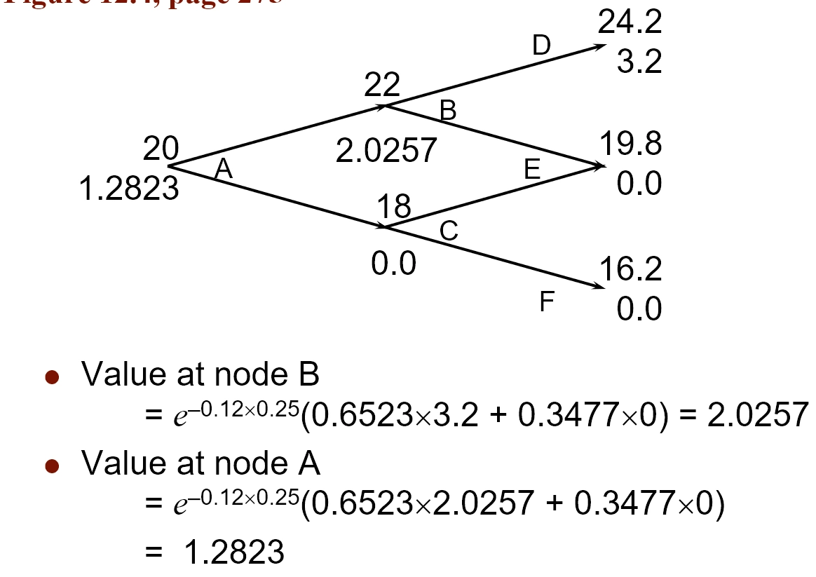
Valuing a European Put Option
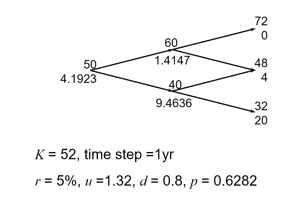
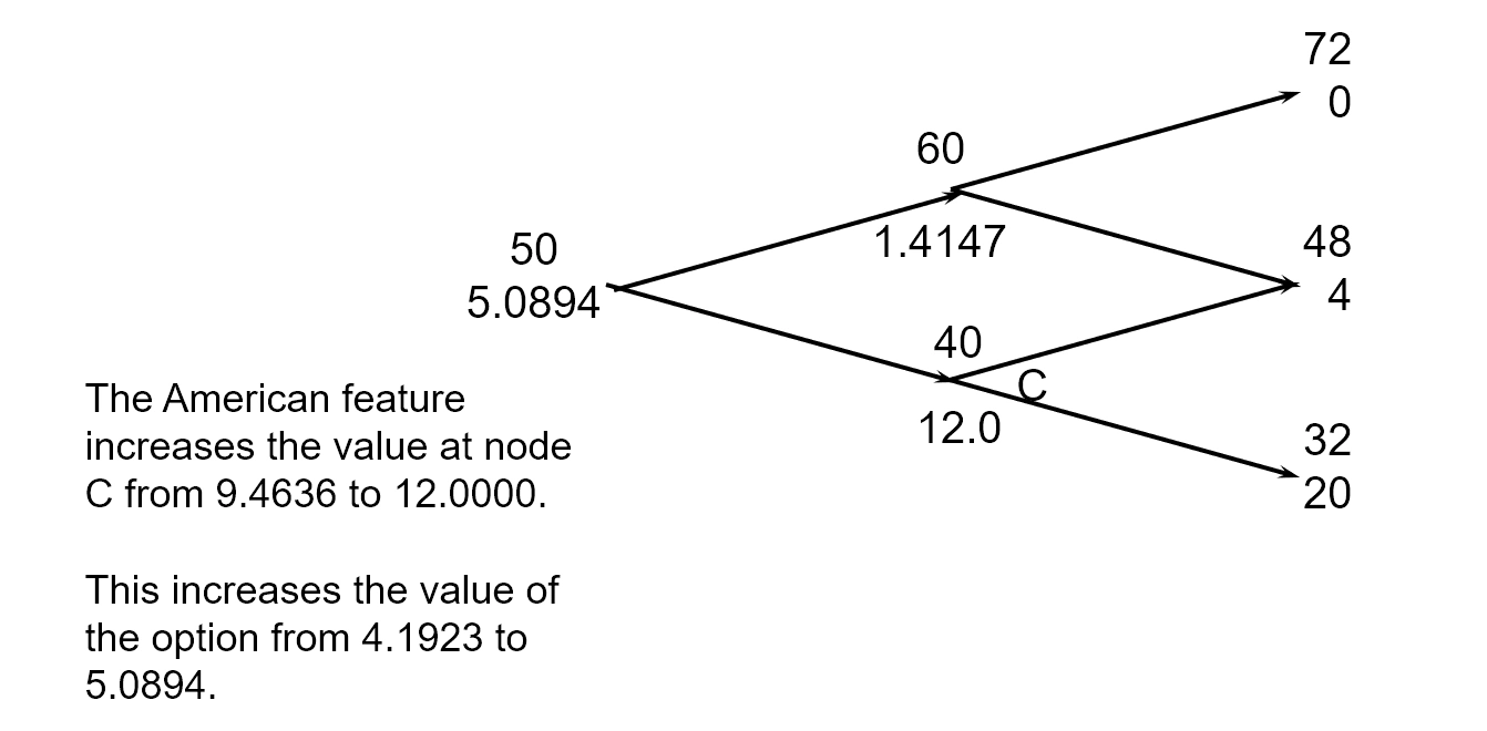
Valuing an American Put Option
Choosing u and d
- Sigma is the annualized volatility
u = e^(sigma sqrt(delta t))d = 1/u = e^-(sigma sqrt(delta t))
Options on Stock Indices, Currencies, Futures
- Same process except p is different
- Probability of an up move
- Cash settlement one day later
- S&P 100 and AMEX Major Market Index are examples of a broad indices
p = (a - d) / (u - d)
- Non-Dividend: a = e^(r * delta t)
- Index with yield q: a = e^((r-q) * delta t)
- Currency with foreign risk-free rate rf: e^((r-rf) * delta t)
- Futures: a = 1
Time Steps
- At least 30 time steps are required for good option values
- DerivaGem allows up to 500 time steps
Chapter 18 - Binomial Trees in Practice (DerivaGem)
- approximate movements in the price of a stock or other asset
- for each small interval of time (delta t), stock moves up u or down d
- tree parameters for a non-dividend paying stock: volatility, risk-free rate, stock price
Custom Derivative Payoff Example
- S0 = 20
- Sigma = 25%
- r = 5%
- T =6mo
- Time step = 3 mo
- Payoff = MAX(S^2 - 400, 50)
- Using the two-step example, we get a price of $103
Put Example Delta Shares Short
- Delta = (2.16 - 6.96) / (56.12 - 44.55) = -0.41 (the payoff from the next step)
- As time passes, delta will change (delta hedging)
Chapter 13 - Black-Scholes-Merton Model
- Assumptions
- The assumption in equation (13.1) implies that the stock price at any future time has a lognormal distribution.
- Volatility on the underlying is known and constant
- price of a European call option as the time step tends to Zero
- mean \mu is the expected return and \sigma is volatility
- Delta S / S is the stock return which is normal distributed
Lognormal Property
Standard deviation:
Therefore the normal distribution, \phi [mean, variance], Is
or
Example
- N = 16%, std = 35%, S0 = $38
- Calculate probability that a european call option with k = %40 and maturity 6 months out will be exercised
- P(S_T > 40)
- Use online distribution calculator to figure it out
Estimating Volatility from Historical Data
- Take observation S_0, S_1, S_n at intervals of Tau years (for weekly data, Tau = 1/52)
- Calculate the continuously compounded return in each interval as:
mu_i = ln (S_1 / S_{i - 1}) - Calculate the standard deviation, s, of the mu_i’s
- Historical volatility estimate is: \sigma \hat = s / (sqrt ( Tau))
- Tau decision: need as many observations as possible
- With daily, lots of noise
- Period has to be big enough period for validity
- Need more than 30 observations
Black-Scholes Formulas
European Call
European Put
d1 variable
d2 variable
The variable mu does not appear in the black-scholes equation. It is independent of all variables affected by risk preference. Consistent with risk-neutral valuation principle.
- N(d2) is the probability of exercising
With dividends, need to substitute the stock price with the stock price minus the dividends paid through the maturity
Implied Volatility
- The volatility that makes the model price the derivative the same as the market price.
- If two options with the same underlying have different implied volatilizes, something might be overpriced/underpriced
Chapter 15 - Options on Stock Indices and Currencies
- Most popular in the U.S.A are S&P 100 (OEX, XEO), S&P 500 (SPX), DOW times 0.01 (DJX), NASDAQ 100 (NDX)
- Contracts are settled on 100 times the index in cash OEX is American whereas the others are European
Example 15.1
- Portfolio Beta of 1.0
- Value is $500,000
- Index at 1,000
- What trade is necessary to provide insurance to prevent value from falling below $450,000
Example 15.2
- Portfolio has Beta of 2.0
- Value is $500,000
- Index at 1,000
- rf = 12% per annum
- dividend yield on both is 4%
- How many put options to purchase on the index at the strike?
How to solve?
- Find relationship of portfolio to index.
- The portfolio return is the value that fell plus the pro-rated dividends that was received
- Then use this return to calculate the situational return on the index and subtract the dividend yield
- Do do this use CAPM formula
- This nominal value on the index is the strike price we want to purchase of the put
- Find number of puts to purchase
- Put options to purchase to cover the initial portfolio:
Beta \* ValueOfPortfolio / (ValueOfIndex * 100)where values are the initial values
- Put options to purchase to cover the initial portfolio:
Currency Options
- NASDAQ OMX
- Used for buying insurance when exposed to FX
- Lower bound is equivalent to european options with dividends
Range Forward
Chapter 16 - Futures options and Black’s Model
- American and expires a few days before the earliest delivery
- When a call futures option is exercises
- The Holder acquires
- A long position in the futures
- A cash amount equal to excess of the futures price at the most recent settlement over the strike price
- The Holder acquires
Example 16.1
- July call option on gold futures with a strike of $12000 per ounce. Exercised when futures price is 1,240 and recent settlement of 1,238. One contract is 100 ounces
- Trader receives: one long July contract on gold and (1238 - 1200) * 100 = 3800.
Example 16.2
- September put option on corn 300 cents per bushel
- exercised when futures is 280 cents per bushel with recent settlement of 279 cents per bushel
- Trader received: long short futures on the corn contract and 21 cents per bushel in cash
Immediately Selling the Future Payoff
- Payoff from call = F - K
- Payoff from put = K - F
Advantages of Future Options over Spot Options
- futures may be easier to trade
- no delivery
- futures and options trade on the same exchange
- futures options may entail lower transaction costs
European Futures Options
- the futures option and spot options are equal at maturity
- spot options are regarded as futures options when valued over the counter
- when futures prices decrease with maturity, American call futures are worth less than the corresponding American call on the underlying asset
- American futures options are never equal to European futures options unless it’s the last day of exercising
Put-Call Parity for European Futures Options
Binomial Riskless Futures Option Pricing
- 1 month out
- 3Delta - 4 = 2 Delta → Long Delta futures of 0.8
- With a risk-free rate of 6%, the value of the portfolio is (2 * 0.8)e^{-0.06/12} = -1.592
- Value of the options must be 1.592 since the value of the futures is 0
The portfolio is risk-less when
Chapter 17 - The Greek Letters
- Delta = change in option price with relation to underlying
- Vega or Lambda: change in option price with relation to underlying implied volatility
- if volatility goes up and price of underlying stays the same, both the put and call options go up in price
- Theta: change in option price with relation to time
- If gamma and delta are 0, then the portfolio is risk-neutral and should be appreciating at the risk-free rate
- Rho: change in option price with relation to interest rate
- Gamma: Change in option’s delta in relation to stock price change (2nd derivative)
- Positive for long puts and calls since if price goes up, delta will go up for call obviously, but also up for put since less short is needed in underlying
Stop-Loss Strategy
- assuming a naked call position
- buying 100,000 shares as soon as price reaches $50
- selling 100,000 shares as soon as price falls below $50
- if the stock fluctuates around the strike price of 50, then this strategy loses lots of money due to buying high and selling low
How Delta-Hedging Works
If we hold a short call position and hold delta shares, why are we doing so? When the underlying’s value goes up, we lose delta in the short call options, but we also gain on the underlying shares.
- delta on a european non-dividend call is N(d1)
- european non-dividend put: N(d1) - 1
- As time to maturity decreases, delta of out the money calls increases, and in the money calls decreases
- Buy high sell low
Example 17.1
- A bank has sold for $300,000 a European call option on 100,000 shares of a non-dividend- paying stock
- S0 = 49, K = 50, r = 5%, s = 20%,
- T = 20 weeks, m = 13%
- The Black-Scholes-Merton value of the option is $240,000
- How does the bank hedge its risk to lock in a $60,000 profit?
Gamma Addresses Delta Hedging Errors Caused by Curvature
- greatest for options at the money
- Tau = portfolio value
- change in gamma = Theta times change in time + 0.5 Tau change in share price squared
Managing Delta, Gamma, and Vega
Gamma and Vega require taking a position in the options themselves.
| – | Delta | Gamma | Vega |
|---|---|---|---|
| Portfolio | 0 | -5000 | -8000 |
| Option 1 | 0.6 | 0.5 | 2.09T11 |
| Option 2 | 0.5 | 0.8 | 1.2 |
What position in option 1 and the underlying asset will make the portfolio delta and gamma neutral? Answer: Long 10,000 options, short 6000 of the asset
What position in option 1 and the underlying asset will make the portfolio delta and vega neutral? Answer: Long 4000 options, short 2400 of the asset
What position in option 1, option 2, and the asset will make the portfolio delta, gamma, and vega neutral? We solve
  −5000+0.5w1 +0.8w2 =0
  −8000+2.0w1 +1.2w2 =0
to get w1 = 400 and w2 = 6000. We require long positions of 400 and 6000 in option 1 and option 2. A short position of 3240 in the asset is then required to make the portfolio delta neutral
Rho
Rho is the rate of change of the value of a derivative with respect to the interest rate
Hedging in practice
- become delta-neutral at least once a day
- whenever opportunities arise, improve gamma and vega
- hedging becomes less expensive as a portfolio gets larger
Greek Letters When Underlying has a Yield
See slide 32 of slide deck 17 (or see page 381)
Futures for Delta Hedging
futures is e^{-(r-q)T} times the position required in the spot contract
Synthetic Option
- take positions that match the greeks of the option
Portfolio Insurance
- Sell enough of the portfolio or index futures to match the delta of the put option (e.g. October 1987)
- As portfolio value increases, delta goes down and so original portfolio is repurchased to some extent
- As portfolio value decreases, more of portfolio is sold
Chapter 22 - Exotic Options
- Packages
- Nonstandard American options
- Gap options
- Forward start options
- Cliquet options
- Compound options
- Chooser options
- Barrier options
- Binary options
- Lookback options
- Shout options
- Asian options
- Options to exchange one asset for another
- Options involving several assets
Packages
- Portfolios of standard options
- Examples from Chapter 11: bull spreads, bear spreads, straddles, etc
- Example from Chapter 15: Range forward contracts
- Packages are often structured to have zero cost
Nonstandard American options
- Bermudan: exercisable on specific dates
- initial lock out period
- strike price changes over life
Gap Options
- Call option pays (ST - K1) when (S > K2)
- Put option pays (K1 - ST) when (S < K2)
- Valuation formula found in Chapter 22
Forward Start Options
- Option starts at a future time T
- Often structured so that strike price equals asset price at time T
- Planning to give employees at-the-money options in each future year can be regarded as a series of forward start options
Cliquet Option
- rules determine how the strike price is determined
- for example, 20 at-the-money three-month options (total life of five years)
- When one option expires, a similar one comes into existence
Compound Options
- An option on an option
- Call on call
- Put on call
- Call on put
- Put on put
- Very sensitive
Chooser Options
- start at 0, mature at T2
- at T1, buyer can choose whether the option is a put or a call
- this is a package
- p = c + e^{-r(T2-T1)}K - S1 e^{-q(T2-T1)}
- At T1, c + e^{-q(T2-T1)} max(0, Ke^{-(r-q)(T2-T1)} - S)
- call maturing at T1 plus put maturity at T1
Barrier Options
- in: option comes into existence only if asset price hits barrier before option maturity
- out: option are knocked out if asset price hits barrier before option maturity
- up: asset price hits barrier from below
- down: asset price hits barrier from above
- eight possible combinations (put or call)
- parity
- c = cui + cuo
- c = cdi + cdo
- p = pui + puo
- p = pdi + pdo
Binary Options
- Cash-or-nothing: pays Q if S > K at time T. Value = e^{-rT}QN(d2)
- Asset-or-nothing: pays S if S > K at time T, or nothing. Value = S0e^{-qT}N(d1)
Lookback Options
- Floating call: Pays
Stock at time T – Stock minimumat time T- Allows buyer to buy stock at lowest observed price in some interval of time
- Floating put: pays
Stock max - Stock at time Tat time T- Allows buyer to sell stock at highest observed price in some interval of time
- Fixed call: pays maximum observed asset price minus strike price
- Fixed put: pays strike price minus minimum observed asset price
Shout Options
- Able to lock in a price once during the life
- Usually pays like a call or a put but also the intrinsic value at the shout time
Asian Options
- Payoff related to average stock price
- average price
Options to Exchange
- One asset for another
- Payoff is price difference between the assets
Basket Options
- option on the value of a portfolio
Mortgage-Backed Securities
- Pass-Through
- Collateralized Mortgage Obligation (CMO)
- Interest Only (IO)
- Principal Only (PO)
Variations of Interest Rate Swaps
- different principles
- different payment frequencies
- floating for floating or fixed for fixed
Compounding Swaps
- Business Snapshot 22.2
- Interest is compounded instead of paid
Complex Swaps
- LIBOR-in-arrears swaps
- CMS and CMT swaps
- Differential swaps
Equity Swaps
- Business Snapshot 22.3
- Total return on equity index is exchanged for a fixed or floating return
Embedded Swaps
- Accrual swaps
- Cancelable swaps
- Cancelable compounding swaps
Other Swaps
- Indexed principal swap
- Commodity swap
- Volatility swap
- Bizarre deals: P&G 5/30 swap
- P&G receiving 5.3% interest on $200M for 5 years semi-annually
- P&G would pay back the 30-day commercial paper rate minus 75 basis points plus spread
- spread = max (0, 98.5 * (5 year commercial constant maturity rate) / (5.78%) - 5 year treasury price) / 100
Chapter 8 - Secularization
- traditionally loans are funded via deposits
- loans can increase much faster than deposits
- Assets are combined and sold in tranches
- Senior Tranche 80% (ABSs) - AAA
- Mezzanine Tranche (15%) - BBB - ABS CDO Created
- Senior Tranche (65%) - AAA (does not convey actual risk)
- Mezzanine Tranche (25%) - BBB
- Equity Tranche (10%)
- Equity Tranche - Not Rated
- Bankruptcies wipe out from equity first
- Asset cash flows go first to senior, then mezzanine, then equity
What Led to the Financial Crisis
- Starting in 2000, mortgage originators relaxed lending standards and created large subprime first mortgages
- demand for real estate and prices rose
- 100% mortgage
- ARMs
- teaser rates
- no income, no job, no assets (NINJAs), ARMs, teaser rates, liar loans, non-recourse borrowing (repossession)
What was not accounted for
- Default correlation increase in stressed market conditions
- Recovery rates are less in stressed market conditions
- Tranche with a certain rating cannot be equated with a bond with the same rating
- BBB tranches used to create ABS CDOs were 1% wide nad had all or nothing distributions
- not the same as the loss distribution for a BBB bond
Regulatory Arbitrage
- capital required to keep for the tranches was less than the mortgages themselves
- mortgage originators: only cared about originating mortgages that can be securitized
- Valuers: under pressure to provide high valuations to keep business
- traders: focused on year-end bonus and not long term
Aftermath of Financial Crisis
- Banks required to hold more equity capital with the definition of equity capital being tightened
- Banks required to satisfy liquidity ratios
- CCPs and SEFs for OTC derivatives
- Bonuses limited in Europe
- Bonuses spread over several years
- Proprietary trading restricted
Chapter 25 - Derivative Mishaps
Losses by Non-Financial Corporations
- Allied Lyons ($150M)
- Gibsons Greeting ($20M)
- Hammersmith and Fulham ($600M)
- Metallgesellschaft ($1.8B)
- Promised client long term supply of oil at certain prices
- Sold hedge at the bottom and then the hedge was useless
- Orange County ($1.6B)
- Robert L. Citron was making excess returns
- Reverse repos
- Borrowed money in short-term and invested in short-term markets
- Took new assets and put them up as collateral to buy in long-term securities
- Procter and Gamble ($90M)
- Shell ($1B)
- Sumitomo ($2B)
- Trader at Sumitomo was trying to recoup losses through copper
Losses by Financial Institutions
- Allied Irish Banks ($700M)
- Amaranth ($6B)
- Barings ($1B)
- Enron’s counterparties (billions)
- Kidder Peabody ($350M)
- LTCM ($4B)
- high leverage
- exposure to 1997 Asian financial crisis and 1998 russian financial crisis
- Midland Bank ($500M)
- Societe Generale ($7B)
- Subprime mortgages (tens of billions)
- UBS ($2.3B)
Chapter 19 - Volatility Smiles
For options with some maturities, the implied volatility versus the strike price makes a smile.