Objectives

Viewpoints

• database user
• database designer
• database manager

Sub-objectives

• SQL
• data modeling
• management
• database management system (DBMS)
• Relational model
• Application programming
• Transaction and concurrency

File-Processing Systems

Disadvantages with File-Processing Systems

• Data redundancy and inconsistency
  • various copies leads to higher storage
• Difficulty in accessing or modifying data
• Integritty problems
  • New constraints require changing the program
• Atomicity problem
  • Difficult to ensure atomic property and to restore state after failure
• Concurrency issues
• Security

Databases

Database Definition

A large and persistent collection of (more-or-less similar) pieces of information organized in a way that facilitates efficient retrieval and modification.

Database Management System (DBMS)

A program (or set of programs) that manages details related to storage and access for a database.

• Data model
• Access control
• Concurrency control
• Database recovery

Scheme Definition

A schema is a description of the data interface to the database

Database Instance Definition

A database instance is a database (real data) that conforms to a given schema ) i.e., the information stored in the database at a particular moment

Levels

• Physical
• Virtual
• External

The Relational Model

A database is a collection of relations (tables). Each relation has a set of attributes (columns). Each attribute has a name and an atomic (indivisible) domain (type). Each relation has a set of tuples (rows). Duplicate tuples are not allowed. Two tuples are duplicates if all their attributes agree.

Data Model

• structure
• operations
• constraints

Schema and Instance

author(aid:int, name:string)
publication(pubid:int, title:string)
journal(pubid, volume)

A database can be displayed tabularly with a table for each relation.1

Integrity Constraints

Tuple-Level

• Domain restrictions (e.g. type string)
• Value restriction: only allow subset of values (e.g. ["Winter", "Summer", "Fall"])

Relation-level

• Superkey: attributes where tuples will never agree on
• Candidate key: minimal superkey (minimal set of attributes that unique identify the tuple)
• Primary key: designated candidate key

Database-level

• Foreign key: an attribute of this relation is the primary key for another relation (Relation one is referencing and the second relation is referenced )
• Foreign key constraints: Foreign key must match the primary key value of a tuple in the referenced relation
• Referential integrity constraints: foreign key cannot be a primary key in the referencing relation

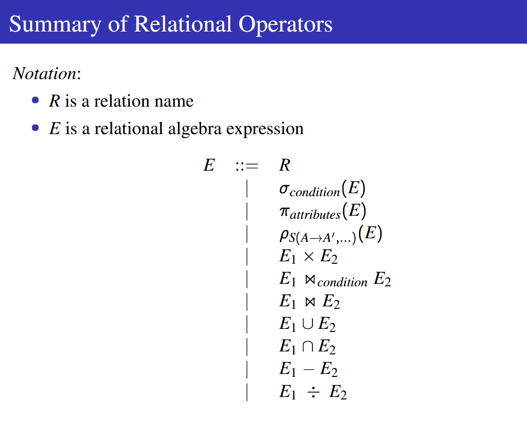
The Relational Algebra

Consists of a set of operators

Operators

• one or two relations as inputs
• single output relation in terms of the input relation(s)
• can be composed to express the definition of a new relation in terms of existing relations

Selection

subset of tuples of a relation and thus schema is the same

• Find teachers who are in the physics department
• conditions include any column of R, comparisons, boolean algebra
• select applies to single row at a time, not many

Projection

• Returns a subset of a relation but only of the specified attributes
• Duplicates are eliminated

Cross Product

• Result has attributes of both input relations
• Result is the tuple for each possible pair from relation one and relation two

Conditional Join

• Perform cross product but join pairs only if the boolean involving attributes from both relations is true

Natural Join

If both relations have the same attribute, then the join will only filter out tuples that don’t have those attributes matching. During the first cross product, duplicate attributes are renamed (e.g. ID, ID -> ID, ID_1) but at the end the duplicated attributes are thrown out.

Set-Based Relational Operators

• Union: Same number of fields and corresponding fields have the same type
• Difference: Returns stuff in first relation not present in second
• Intersection: Return stuff in both rrelations
• Division: Attributes of second relation must be a subset of the first. Inverse of product. Useful for all. Example (which tuples of X always references Y but returns a new tuple without the attributes in Y).

Summary of Relational Operators

Finding the maximums of a relation

To do this, we find all values in the relation that are smaller than values in itself. Now that we have all the smaller values, we just need to remove them from the original table. We are left with values equal to the maximum.

project val (T) - project t1.val (T t1 join T t2 if t1.val < t2.val)

Algebraic Equivalences

Relational Completeness

The Relational Calculus

SQL - Structured Query Language

KEYWORD (statements is implied)

• SQL Data Manipulation Language (DML)
  • SELECT for queries
  • INSERT, UPDATE, DELETE modify the instance of a table
• SQL Data Definition Language (DDL)
  • CREATE, DROP modify the database schema
• SQL Data Control Language (DCL)
  • GRANT, REVOKE enforce the security model

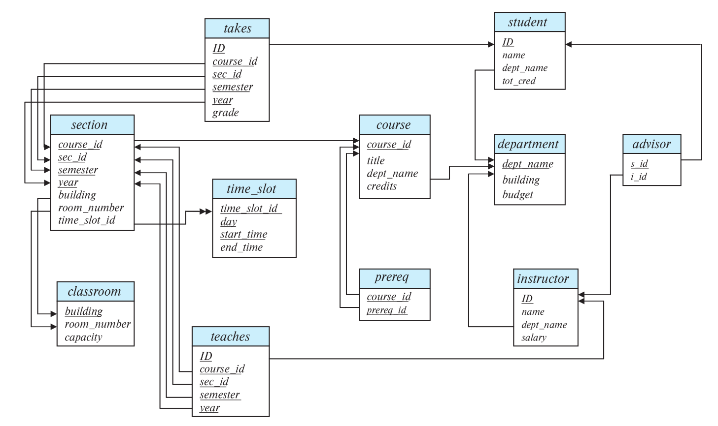
Schema used for Examples

SQL interpreter

Data Types

• integer or int (32 bit or 4 byte)
• smallint (16 bit or 2 bytes)
• numeric(p, q): p digit numbers with q digits to the right
• real, double precision:
• float(n): user-specified precision of at least n digits
• char(n): fixed length character strings (n is length)
• varchar(n): variable length character to a max length of n
• date: describes year, month, day
• time: describes an hour, minute, second
• timestamp: describes a date and time
• interval: allows date/time computations

Tables

create table r
  (A1 D1, ..., An, Dn),
  (integrity-constraint-1),
  ...
  (integrity-constraint-k),

r: relation, A: attribute, D: data type

integrity-contraints:

primary key (A1, ..., An )
foreign key (Am, ..., An ) references r2

Queries

SQL allows duplicate tuples in relations as well as in query results. need to use the distinct keyword after select.

SELECT [distinct] dept_name, salary from instructor

[OPTIONAL]

To return all attributes, use an asterisk (*)

Arithmetic Expressions

You can operate on the data through the select call itself. For example, if we wanted the monthly salary instead of an annual one:

select ID, name, salary/12 as monthly_salary from instructor

Filtering (Where)

select name from instructor where dept_name = ’Comp. Sci.’

• logical connectives: and, or, and not
• comparison operations: <, <=, >, >=, =, and <> (inequality)
• comparisons can be applied to results of arithmetic expressions

Select Cross Product

Performs Cross product by specifying multiple relations

select * from instructor, teaches

Use where to join and remove duplicate attributes.

select * from instructor, teaches where (instructor.ID = teaches.ID and instructord.dept_name = 'Comp. Sci' and year = 2017)

FROM Inner Join

... from instructor inner join teaches on instructor.ID = teaches.ID...

If attributes have the same name, then both will show up with a relation. prefix

FROM Natural Join Clause

select * from instructor natural join teaches

Be careful since this does it to all attributes. For specific attributes, use using

select * from T join S using(A)

SELECT as

Renaming the attribute in the query result

select T.ID, T.name from instructor as T, instructor as S where T.salary > S.salary and S.ID = '12121'

String Operations

• ‘5"6’ (allows double quotes)
• ‘Datebase’ = ‘database’ (false)
• DBMS might not differentitae (MYSQL)
• concat
• to upper or to lower
• string length, extracting substrings, etc.

WHERE like

• %: match any substring
• _: match any charater (one)
• escape using escape '%' or escape '_'

WHERE attribute like '%pattern%'

ORDER

select name from instructor order by name asc   -- default is asc
select name from instructor order by dept_name, name  desc

Union

select course_id
from section
where semester=’Fall’ and year=2017
union
select course_id
from section
where semester=’Spring’ and year=2018

-- union all

select course_id
from section
where semester=’Fall’ and year=2017
union all
select course_id
from section
where semester=’Spring’ and year=2018

Aggregate Pt. 1

• avg: average value
• min: minimum value
• max: maximum value
• sum: sum of values
• count: number of values
  • count (*) to count number of tuples Usage SELECT count(attribute), ...

Group by: group tuples into another attribute.

select dept_name, avg(salary) from instructor group by dept_name having avg(salary) > 25000

The having condition applies on each group and not on the aggregation. The having applies before the select returns but after the grouping.

Null: null indicates unknown or missing data.

Comparing null with anything else always results in unknown even with null.

Unknown always takes precedence.

Use is null for a null comparison

Subqueries

Use ( ) to use a temorary relation

Table Subqueries

select dept_name, avg_salary
from (
  select dept_name, avg(salary) as avg_salary from instructor group by dept_name
) where avg_salary > 42000

select max (tot_salary) from (
  select dept_name, sum(salary) as tot_salary from instructor group by dept_name
)

Scalar Subqueries

A query that returns a single tuple.

select name from instructor where salary >
   (select avg(salary) from instructor)

Set Membership

Subquery can also be a hardcoded set

x in (subquery) /* intersect */
x not in (subquery) /* except */
select distinct name from instructor where name in (’Mozart’, ’Einstein’)
select distinct name from instructor where name not in (’Mozart’, ’Einstein’)

<> means not equal

All Clause

select name from instructor where salary >
  all (select salary from instructor where dept_name = 'Comp. Sci.')

Some (at least one) Clause

select name from instructor where salary >
  some (select salary from instructor where dept_name = 'Comp. Sci.')

Exists Clause

Can also use not exists

select course_id from section as S where semester = 'Fall' and year = 2017 and
  exists (select * from section as T where semester = 'Spring' and year= 2018
  and S.course_id = T.course_id)

Test Non-Empty Relations

Triple query.

Assert inner query is non-empty (not exists) where inner query does a search based on condition 1 which also asserts it satisfies condition 2 which could be another query.

Find all students who have taken all courses offered in the Biology department.

return student if for all biology courses available student has taken that course. -> return students where the following relation is empty (all bio courses except the ones the student has taken)

Unique

Returns true if subquery contains no duplicates (one find). Add not before unique for “at least twice”

select * from course as T where unique
  (select * from course as R where T.course_id = R.course_id and R.year = 2017)

Correlated Subqueries

For each tuple obtained from the outer query, compute the inner query. Need to use the lateral prefix to do so.

select name, salary, (select avg(salary)
  from instructor where dept_name = S.dept_name) as dept_avg
  from instructor as S

select name, salary, dept_avg from instructor T,
  lateral (select avg(salary) as dept_avg from instructor S
              where T.dept_name = S.dept_name)

With Clause

with temp_relation (list_of_attributes) as (subquery)

Find all departments where the total salary is greater than the average of the total salary at all departments

with dept_total (dept_name, value) as (select dept_name, sum(salary)
            from instructor group by dept_name),
        dept_total_avg (value) as (select avg(value) from dept_total)

select dept_name from dept_total, dept_total_avg
    where dept_total.value > dept_total_avg.value

Data Modifications

alter table r add attribute data_typ

Existing tuples in r will have null as the value for the new attribute

alter table r drop A

• Not supported on many databases like SQLite

alter table r rename column old_name to new_name

alter table r modify A data_typ

Deleting a Table

drop table instructor

Removing from Table

Remove all:

delete from instructor

delete from instructor where dept_name= ’Finance’

delete from instructor where salary < (select avg(salary) from instructor)

Insertion

insert into course values (’CS-437’, ’Database Systems’, ’Comp. Sci.’, 4)

insert into course (course_id, title, dept_name, credits) values (’CS-437’, ’Database Systems’, ’Comp. Sci.’, 4)

insert into student values (’3003’, ’Green’, ’Finance’, null)
insert into student values (’3003’, ’Green’, ’Finance’) /* omitted values will be null */

Inserting into new table from another based on some condition. Note that without a primary key on the student table, there would be a infinite tuples added.

insert into instructor select ID, name, dept_name, 18000 from student
  where dept_name = ’Music’ and total_cred > 144

Updates

update instructor set salary = salary * 1.05;

update instructor set salary = salary * 1.05 where salary < 70000;

update instructor set salary = salary * 1.05 where salary < (select avg (salary) from instructor);

Update instructor salaries based on how much they make (multiple queries):

update instructor set salary = salary * 1.03 where salary > 100000;
update instructor set salary = salary * 1.05 where salary <= 100000;
/* alternative using case */
update instructor set salary = case
    when salary <= 100000 then salary * 1.05
     else salary * 1.03
  end

SQL Intermediate Topics

Check Constraints

create table department (
  ...
  budget numeric (12,2) check (budget > 0),
  ...
)

Foreign Key Contraints

create table instructor (
  ...
  dept_name varchar(20)
  ...
  foreign key (dept_name) references department )

Deleting in Referenced Relation

When creating a table, we can use the references R on delete set null

Cascade: on delete cascade rows referencing key also get deleted

Views

virtual table

create view faculty as select ID, name, dept_name from instructor

We can use views to hide data

Modifying Views

create view instructor_info as select ID, name, building from instructor, department where instructor.dept_name = department.dept_name;
-- insert into instructor_info values('69987', 'White', 'Taylor'); -- won't work

Updateable Views

Access Control

Roles

Indexes

• An index is an auxiliary persistent data structure
  • Search tree (e.g., B+-tree), lookup table (e.g., hash table), etc

create index ins_name_index on instructor (name);
create unique index ins_name_index on instructor (name);
drop index ins_name_index

Typically the index already exists on primary key and unique constraints.

SQL Relational Division

TODO: double check if this is correct.

Assumes model is distinct (primary key). If model was not distinct, you would have to add the distinct keyword in the subquery as well as the ending count.

SELECT maker FROM (SELECT maker, model FROM Product A join Printer B USING(model) WHERE color=True) group by maker HAVING COUNT(*) = (SELECT COUNT(*) FROM Printer WHERE color=true)

SQL Drivers

Prepared Statements

Compile once and reuse multiple times. Avoids SQL Injection.

Metadata Features

Functions and Procedures

create function func_name(param_decls)
returns return_type
create procedure proc_name(param_decls)
call proc_name(params)
set variable = call func_name(params)

Procedures do not have return values, rather they use out parameters. Additionally, parameters can modify whereas functions are read only. Procedures can call other procedures and functions but functions cannot call functions nor procedures. You can use functions as if they are tables/views but

Triggers

Event-Condition-Action

create trigger timeslot_check after insert on section
referencing new row as nrow
for each row
/*time_slot_id not present in time_slot */
when (nrow.time_slot_id not in (select time_slot_id from time_slot))
begin
  rollback
end;

• Can be before or after
• For each statement is also possible but only applies to after triggers
  • Useful for SQL statements that update a larger number of rows

Ranking

select ID, rank() over (order by (GPA) desc) as s_rank from student_grade order by s_rank;

select ID, dept_name, rank() over (partition by dept_name order by (GPA) desc) as dept_rank from student_grade order by dept_name, dept_rank;

Windowing (Moving)

select year, avg(num_credits) over (order by year rows 2 preceding) as avg_total_credits from tot_credits;

select year, avg(num_credits) over (order by year rows unbounded preceding) as avg_total_credits from tot_credits;

select dept_name, year, avg(num_credits) over (partition by dept_name order by year rows between 2 preceding and current row) as avg_total_credits from tot_credits_depth;

Pivoting

• a cross-tabulation view of tables

Rollup and Cube

• multidimensional data aggregation

Recursion

with recursive rec_prereq(course_id, prereq_id) as (select course_id, prereq_id from prereq union select rec_prereq.course_id, prereq.prereq_id from rec_prereq, prereq where rec_prereq.prereq_id = prereq.course_id) select * from rec_prereq;

Entity-Relationship Model

Database Design

Understand the real-world domain being modeled

• E-R model

Translate the specification to the data model of DBMS

• The relational model

Complex Attributes

• Primary key: underlined
• Composite attributes can be shown by indenting the individual attributes that make it up (nestable)
• Use brackets for multi-valued attributes
• Use ( ) suffix to state that the attribute is derived

Mapping Cardinality

Participation

Use a double line to show that all values are participating and use single line for partial participation.

Primary Keys in E-R Model

Weak Entity Sets

A weak entity set is one whose existence is dependent on another entity, called its identifying entity. An entity set that is not a weak entity set is termed a strong entity set.

Removing Redundant Attributes in Entity Sets

• identifying entity sets
• adding attributes to entity sets
• forming the relationship sets among the various entity sets

Specialization

Overlapping Specialization

Use separate arrows

Disjoint Specialization

One arrow from multiple tables

Completeness Constraints

Total specialization: Each entity in the higher-level entity set must be present in at least one lower-level entity set. Requires annotating an arrow.

Partial specialization (default): Membership of a lower-level entity set is not required

Common Mistakes

• use of primary key of an entity set as an attribute of another entity set instead of using a relatioship

E-R Diagram to Relational Tables

• Each entity set maps to a new table
• Each relationship set maps to a new table
• Each simple and single-valued attribute maps to a new column

Schema Refinement: Dependencies

Example

Similar to a question in assignment 2

See slides

Single-Table Schema

• update problems (how to update values of a single column)
• insert problems (adding new subset of tuple)
• delete problems
• likely increases space requirements

Too many Tables

If there are too many tables, the information of relationships is lost

Functional Dependencies: Armstrong’s Axioms

Two ways, first is armstrong’s axioms

Reflexivity

SIN, EName -> EName

Augmentation

If X is a subset of Y, then X -> Y.

SIN, Z -> EName, Z

Transitivity

X -> Y, Y -> Z => X -> Z

Union Rule

X -> Y, X -> Z => X => YZ

Decomposition

X -> YZ => X -> Y, X -> Z

Function Dependencies: Attribute Closure

https://littleflowercollege.edu.in/upload/e_contents/files/187d8c7967172ef5cc75d9b2a709d6cf.pdf ?

Schema Decomposition

Lossless Decomposition

A decomposition {R1, R2} of R is lossless if and only if the common attributes of R1 and R2 form a superkey for either schema, that is

Dependency-preserving Decompositions

If we have functional dependencies, we should be able to still prove those dependencies valid without having to join.

Boyce-Codd Normal Form (BCNF) Decomposition

Informally, a relation schema R is in BCNF if and only if any group of attributes in R that functionally determines any other attributes in R functionally determines all attributes in R , i.e., that group of attributes is a superkey of R

Algorithm:

• Find a BCNF violation
• Decompose the relation into two relations, one being the premise + consequence, the other being premise + attributes not determined

Third Normal Form (3NF)

Minimal cover:

1. Every RHS of a dependency in F is a single attribute
2. There does not exist an FD X -> A in F such that the set F - {X -> A} = F. (no redundant FD)
3. There are no redundant attributes in the LHS set of a FD in F

Transactions

Transaction

A transaction i consists of r_i[x] and w_i[y] and c_i

Execution History

A database is a shared resource that is accessed by many users and processes. If data is accessed or modified concurrently, the information may be outdated or one of the modifications will be lost.

Step 1: check if both transaction histories are over the same set of transactions

Step 2: check if all conflicting pairs (reads and writes for same attribute from different transactions) are in the same order (< or >).

Serial Execution HIstories

For a given transaction history, a transactions operations must be consecutive and operations from different transactions may not be interleaved.

Serial History

Example:

T₁, T₂, T₃

SQL Isolation Levels

Indexing

• Tables of a database are stored in blocks (containing multiple rows) on disks
  • Caching is used (memory buffer pool, writing dirty blocks to disk)
• Sequential reads are faster than random reads
• Indexes can be used to reduce number of blocks read from possibly all to just a few to access a specific row
• Indexes can be used to speed up the access of a range of rows
• Primary keys are always indexed

Index Structure

Transaction Processing

Concurrency Control - Isolation

• Pessimistic - assume conflicts will occur and prevent them
  • Two-phase locking (2PL)
  • Timestamp ordering
• Optimistic - assume that conflicts are rare and run transactions and fix problems that occur

Locking

Shared (read) locks and exclusive (write) locks.

• a transaction that wants to read an object must acquire a shared lock (S mode) on that object
• a transaction that wants to modify an object must acquire an exclusive lock on that object
• object can be locked by multiple shared or only once as exclusive
• not enough for transactions that were meant to preserve a condition such as two objects being the same value

Two-Phase Locking

In phase one, transaction obtain locks and do not release locks. The lock point is when the final lock has been obtained. In phase two, transactions release locks and do not obtain locks. Two phase locking guarantees a conflict-serializable schedule.

Cascading Aborts

If a transaction has read uncommitted data read by a transaction that has aborted, it must abort itself.

Deadlocks

Gradual lock release?

Recovery - Atomicity and Durability

Naïve Approaches

• Force (writes must be reflected on disk when a transaction commits)
• No Steal (flush to disk only at commit)

Logging

• Write to disk just before (WAL: write ahead logging) an object is modified

<T_i, start>
<T_i, X, old_value, new-value>
<T_i, commit> or <T_i, abort>

Checkpointing

Shortens the amount of log that need to be undone or redone when a failure occurs

1. Output onto stable storage all log records currently residing in main memory
2. Output to the disk all modified buffer blocks
3. Output onto stable storage a log record of the form <checkpoint L>, where L is a list of transactions active at the time of the checkpoint

Data Analytics: Warehousing and Mining

Online Transactional Processing (OLTP)

• simple queries
• many short transactions making small changes
• Systems tuned to maximize throughput of concurrent transactions

Data Analytics

the processing of data to infer patterns, correlations, or models for prediction. Used to make business decisions.

1. Gather data
   • Extraction-transform-load
2. Generate aggregates and reports summarizing data
3. Build predictive models

Data Warehouses

Creating and Maintaining a Warehouse

• Extract: queries
• Clean: delete or repair tuples
• Transform: reorg
• Load: populate the warehouse tables

Warehouse Schemas

• Fact tables
• Dimension tables: additional tables for each fact tables
• Measure attributes: value based
• Dimension attributes: relation based

Big Data

Very large volumes of data being collected. Web logs were an early source of data.

MapReduce

• Map
  • User-defined functions
  • Process input key/value pairs
  • Intermediate key/value pairs
• Reduce
  • User-defined functions
  • Intermediate key/value as inputs
  • Merges values for a key

Hadoop

• Develoepd by Yahoo!
• Hadoop distributed file system (HDFS)
  • Multiple data nodes
  • Name nodes store list of block identifiers and machines that have a copy of the block

Apache Spark

• Better for iterative computations
• Fault-tolerant and scalable

Reliable Distributed Dataset (RDD)

• Resilient: if data in memory is lost, recreate
• Distributed: stored in memory across cluster
• Dataset: from a file on HDFS or programmatic

Lineage information retained to reconstruct lost data. Lineage is stored as an object and stored persistently.

Caching

Transformation and Action

NoSQL Systems

Many new application do not require full machinery that relational DBMS’s provide; more so web-based.

• Specialized
  • Column (BigTable)
  • Key-value (DyanmoDB)
  • document (MongoDB)
  • graph (Neo4J)
    • Graph DBMSs are transitioning from NoSQL systems to systems implemented on top of RDBMSs
• Objectives
  • Simplicity (schema-less)
  • Scalability and performance
  • Flexibility for the programmer

CAP Theorem

Distributed data store, only 2 of 3 are ensured

• Consistency
  • All clients always have the same view of data
• Availability
  • Each client can always read and write
• Partition tolerance
  • System works well despite network partitions

Example, two nodes can’t communicate with each other, a write is done one node one and a read is done on node 2. What should node 2 do? Return inconsistent data or stay unavailable.

NoSQL trades consistency for higher availability.

• Database community value consistency (ACID)
• Distributed systems value uptime

Strong vs. Eventual Consistency

• Strong (ACID)
  • All nodes hold the same values
• Eventual
  • Nodes may hold different values but will catch up

Key-Value Stores

Key = unique id, Value = text, binary data, structured data, etc.

• Simple queries
  • Put(key, value): inserts a (key, value) pair
  • get(key): returns value associated with key
  • get_range(key1, key2): { (key, value) }

Amazon DynamoDB

• Data model (key, structured value)
  • Simple queries on key and attributes
  • key is hash or hash and range

MongoDB

• JSON documents
• db.collection.function (JSON expression)

Google BigTable

• Distributed, multi-dimensional, persistent, sparse, sorted map
• Data model: { row and column }
• Transactional atomicity only for single row update

Graph DBMSs

• Many applications (Fraud detection, recommendation engines, AI knowledge gaps, social networks)

Neo4J

• Property graphs
  • Vertices, edges, labels, and properties
• Linked list on disk