BU 473 Investment Management
Bruce Everitt
Table of Contents
Asset Classes and Financial Instruments
Real Assets Versus Financial Assets Real Assets Has productive capacity Financial Assets
- Claims on real assets
- Do not directly contribute to productive capacity
- Fixed-Income Securities
- Equity
- Derivatives
- Other Investments
- Currency
- Commodity and derivative markets
- Financial Markets and the Economy
- Informational role
- Collective judgment determines stock prices
- Consumption timing
- Separate decisions concerning that otherwise would be imposed by current earnings
- Allocation of risk
- Risk preferences
- Agency Problems
- Tying compensation to stocks
- Monitoring from board of directors
- Monitoring from large investors and security analysts
- Takeover threat for poor performers
- Takeover threat for poor performers Financial Markets
- Money Market
- Short-term securities (< 1 year)
- Capital markets
- Long-term bond
- Equity markets
- Derivative markets
- The Money Market
- T-Bill Yields
- Bank-discount method
- Based on par value (face value) as a denominator and 360 days in a year
- Bond-equivalent yield
- Yield is computed based on current price or the purchase price as a denominator and 365 days in a year
- T-Bill Yields
- Commercial paper
- Bonds issued by highly rated companies Bankers’ Acceptances
- Second only to T-bills in terms of default security
- Canadian Dealer Offered Rate (CDOR)
- Bank guarantees that the debt obligation will be fulfilled
- Inflation-Protected Bonds – TIPS or RRB
- Taxable vs. Tax-Exempt Bonds
r * (1-t) > rm
- rm: municipal bond rate Corporate Bonds
- Semi-annual interest payments
- Callable
- Issuer can exercise the call option to buy the bond back
- Poisoned put
- Forces takeover to buy the bond
- Retractable and extendible
- Modifying the maturity date
- Convertible
- Bond holder can convert bond to equity
- Common Stock eQuity
- Residual claim
- Limited liability
- Dividend yield
- Annual dividend / stock price as a percent
- Capital Gains
- P – C
P-E ratio
What is should be versus what it is. Payout ratio over (ke – g). Or (1- retention ratio) / (ke – g) = (1-r)/(k_f+β(mrp)-g)
Sustainable growth: based on what is retained, times the return on earnings?
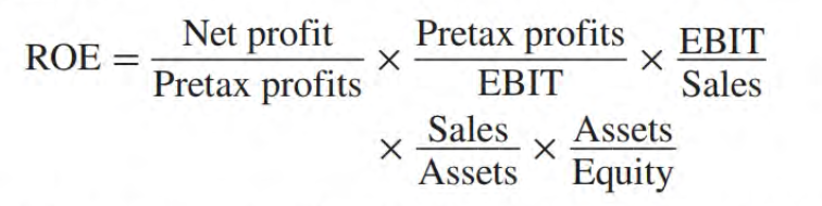
ROE = Earnings / Book Value
Preferred Stocks
Cumulative means that missed payments are still owed. With non-cumulative preferred shares, company does not have to pay the missed payments ever.
Shares become voting at default payment to preferred shares
Income Trusts
- Usually stable revenues
ADR
- American Depository Receipts
- Trade foreign companies within the USA
Indexes
- S&P/TSX
- S&P/TSX 60 Index
- S&P/TSX MidCap and SmallCap
- S&P/TSX Venture Index
The DOW is price-weighted (not value weighted) and it’s divisor accounts for stock-splits
- price-weighted is where you take the sum of prices and divided it by a divisor (given)
- the return of a price-weighted index is based of the index and not the individual returns
Futures vs. Options
- Future: obligation, option: right
Securities Trading
How Firms Issue Securities
- Prospectus
- Preliminary registration statement filed with the Securities and Exchange Commission
- Initial Public Offerings
- The primary market is where new securities are issued for the first time, while the secondary market is where previously issued securities are traded between investors.
- Road show to publicize new offering
- Bookbuilding to determine demand
- Degree of investor interest provides valuable pricing information
- Underwriter bears price risk
- IPOs are commonly underpriced
- Some IPOs are well overpriced
- Facebook
- Retail investor interest lasts only for 2 days. Institutions always drive volume
- Facebook
- IPOs are commonly underpriced
over-allotment: when all equity is sold so banks want more to sell
underwriter takes the risk
Types of Orders
- Market order: buy or sell
- price-contingent order:
- Limit buy (sell) order to buy at below (above) specified price
- large order filled at multiple prices
Trading Strategies
- Algorithmic trading
- High-frequency trading
- HIgh volume low profit
- Dark pools
- private trading systems in which participants can buy or sell large blocks of securities without showing their hand
Trading Costs
- Explicit cost
- Commission
- Implicit costs
- Dealer’s bid-ask spread
- Price concession an investor may be forced to make for big quantities
- Buying board lots is prioritized than fractional
Trading with Margin and Short Sales
Margin is collateral that is on the brokerage platform
- total funds is the collateral (equity) plus the debt
Initial margin is usually 50%
- Maintenance margin
- When equity is 30%, add more money
- How far can a stock price fall before a margin call?
P = Purchase Price * (1 - initial margin) / (1 - maintenance margin)
P =(Sell Price * (1 + initial margin)) / (1 + maintenance margin)
equity required = initial margin * value - value + borrowed = 1,800
equity total required = 0.6 * value
Leverage
Multiplier effect
Short Sale
Benefit when price goes down.
Insider Trading
- Someone trading on information not profitable
- Most common is spouse of someone on legal team
Debt Yields
- Bank Discount Yield
- Discount / Face Value * 360 / Maturity Days
- Price based on a bank discount yield
- Face value - face value * yield * (days / 360)
- If based on a bond yield, use 365 days
- Holding period return
- The delta you get back divided by the price you paid for it
- Effective annual yield
- The holding period return but compounded to a year (365)
- Suppose a holding period return is 3% for 90 days, what is the effective annual yield?
- (1 + 0.03) ^ (365 / 91) - 1 = 12.59%
- Bond equivalent yield
- Ignore effect of compounding (multiply annual holding period return)
- 365 day yield but linear instead of compounded
- Holding period return linearly increased to a year
- yield = 3% / (90 / 365)
- Current yield
- Coupon Payment / Price
Questions
A t-bill has a bank discount yield of 6.81% based on the ask price and 6.9% based on the bid price. The maturity of the bill is 60 days. Find the bid and ask prices of the bill.
Convert 6.81% and 6.9% for 60 days. 360 days in a year
- 1000 - 1000 * 0.0681 * 60 / 360 = 988.65
- 1000 - 1000 * 0.069 * 60 / 360 = 988.5
- Therefore the bid-ask spread is just $0.15
A u.s. treasury bill with 90-day maturity sells at a bank discount yield of 3%.
- a. what is the price of the bill?
- b. what is the 90-day holding period return of the bill?
- c. what is the bond-equivalent yield of the bill?
- d. what is the effective annual yield of the bill
answer
- a. 1000 - 1000 * 0.03 * 90 / 360 = 992.5
- b. 1000 / 992.5 - 1= 0.756%
- c. 365 days instead of 360: yield = 0.756% * 365 / 90 = 3.06%
- d. 1.00756 ** (365/90) - 1 = 3.1%
Purchase 300 shares of GameStart at $40/share. Borrows $4,000 from her broker to help pay for the purchase. Interest rate on loan is 8%.
a. What is the margin of Dei’s account when she first purchases the stock? b. share price falls to $30 per share at year end, what is the remaining margin (equity) on the account? c. margin requirement is 30%, will a margin call occur? d. What is the rate of return?
answer
a. (300 * 40 - 4,000) / 300 * 40 = (12,000 - 4,000) / 12,000 = 66.7% b. 30 * 300 - 4,000 * 1.08 = 4,680 c. 4680 / 9000 = 52% > 30%, so no d. (4680 - 8000) / 8000 = -41.50%
Short sell 1000 shares of GameStart at $40 per share. Initial margin was 50%. Price rose $10. Stock paid dividend of $2.
a. What is remaining margin? b. 30% margin requirement c. rate of return?
answer
a. Initial equity is 50% * 40,000 = 20,000. Final equity is 20,000 + (40 - 50 - 2) * 1000 = 8,000 b. 8000 / (50 * 1000) = 16%, so yes c. (8000 - 20000) / 20000 = -60%
Consider the following limit order. The last trade was at $50.
….
a. market buy for 200 shares, what price will it be filled at? b. at what price would the next market order be filled?
Investment Companies
- Mutual funds
- Record keeping and administration
- Pool everyone’s money and invest
- Professional management
- Lower transaction costs
- Net Asset Value (market value - liabilities over shares outstanding)
- Unit investment trusts
- REITS
- Real Estate Investment Trusts
- Hedge funds
- Private investors pool assets to be invested by fund managers
- Closed-end funds
- Do not redeem or issue shares
- Constant shares outstanding
- Investors cash out by selling to new investors
- Priced at premium or discount to NAV
- Open-end
- Stand ready to redeem or issue shares at NAV
- Priced at Net Asset Value
- NAVn = NAV_0[(1 + r)(1 - MER)]^n
- Management Expense Ratio
Mutual Fund Investment Policy
- Money market funds
- Invest in money market securities such as commercial paper, repurchase agreements, or CDs
- Equity funds
- Invest primarily in stock
- Sector funds
- Concentrate on a particular industry or country
- Bond funds
- Specialize in the fixed-income sector
- International funds
- Global and emerging market
- Balanced funds
- Designed to eb candidates for an individual’s entire investment portfolio
- Asset allocation and flexible funds
- Hold both stocks and bonds
- Engaged in market timing; not low-risk
- Index funds
- Tries to match the performance of a broad market index
- Liquid alternatives
- ESG funds
- screened against environmental, social, and governance factors
Fee Structure:
- Management Fees and Operating Expenses
- Front-end load
- Back-end load
- Trailing Commissions
Exchange Traded Funds
- Mirrors an index
- Trades like a stock
- Lower costs
- Tax efficiency
Hedge Fund Strategies
- Directional
- Bets that one sector or another will outperform other sectors
- Non-directional
- Buy one type and sell another
- market neutral
- Statistical arbitrage
- etc
High-Frequency Strategies
- Electronic news feeds
- Cross-market arbitrage
- Electronic market making
- Electronic “front running”
Examples
- An open-end fund has a net asset value of $10.70 per share. It is sold with a front-end load of 6%. What is the offering price?
- $10.70 after offering price, so offering price = 10.70 / 0.094 = 11.38
The offering price is 12.30 with a front-end load of 5%. What is the NAV? NAV = 12.30 * 0.95 = $11.69
You purchased 1,000 shares at $20 with a front-end load of 4%. Securities increased in value by 12%. There is a 1.2% expense ratio. What is the rate of return?
OFF = 20 / 0.96 = 20.83
Final value = 20 * 1.12 * (1 - 0.012) = 22.13
Rate of return = 22.13 / 20.83 - 1 = 6.24%
- Loaded-up fund has an expense ratio of 1.75%. Economy Fund has a front-end load of 2% but an expense ratio of 0.25%. Assume rate of return is 6% before any fees.
- LU = 1000 * 1.06 * (1 - 0.0175) = 1041.45 -> 4.1%
- EF = 1000 * (1 - 0.98) * 1.06 * (1 - 0.0025) = 1036.20 -> 3.62%
Risk & Return
- Rate of return on zero-coupon bond; r = (100/Price) - 1
- r = (FV/PV)^(1/m) - 1
- Annual Percentage (Posted) Rate (APR)
- Effective annual rate (EAR):
- Takes into consideration the effects of compounding
- (1 + APR/n)^n - 1
- Example
- APR of 4.5%, m = 4
- 100((1 + 0.045/4)^4 - 1) = 4.58%
- What if you want 4.58%?
- Bank A: 4.58% APR, m = 1
- Bank B: 4.5%, m = 4
- Bank C: APR if compound is 12?
- 12 * (1.0458 ^ (1/12) - 1) = 4.4867%
- Continuous compounding
- FV = euler’s constant ^ (rt)
- For a EAR of 4.58%, ln (1 + 4.58%) = r -> r = 4.475%
Interest Rates and Inflation Rates
- Nominal rate is the growth of your money = 11.5%
- Next year, you get 1.115
- Coffee is $1 today, but given an Average annual rate of inflation of 3.5%, the coffee will be 1.035.
- You could buy 1 coffee now and 1.077 next year
- Change in purchasing power (PP) = 1.077 / 1 - 1 = 7.7%
- Fisher equation: N approxEqal to real return + inflation
- Equilibrium rate of return
RIsk and Risk Premium
- Holding Period Return = (enter price - enter price + dividend) / (enter price) = Capital Gain Yield + Dividend Yield
- E(r) = sum of probability of state + return if state occurs
- Variance:
- Standard Deviation (STD)
| State | Prob. of State | r in State | Weighted r | Var |
|---|---|---|---|---|
| Excellent | .25 | 0.3100 | (25)(.31) | (3.1% - 9.76%)^ (.25) |
| Good | .45 | 0.1400 | (.45)(.14) | (14% - 9.76%)^ (.45) |
| Poor | .25 | -0.0675 | (.25)(-0.0675) | (6.75% - 9.76%)^ (.25) |
| Crash | .05 | -0.5200 | (.05)(-.52) | (-5% - 9.76%)^ (.05) |
| Total | 1 | N/A | 9.76% | 0.038 |
STD = sqrt(0.038) = 19.49%
Based on a normal distribution, we can expect a return of 9.76% +- 19.49% 68% of the time.
Risk: likelihood of something happening and magnitude
STD gives us both the magnitude and the likelihood
Look at historical returns, and calculate the STD of those returns to get the
Skewness: positively skewed means a tail on the right
Kurtosis: how normally distributed data is (fatness of the curve)
Calculating the STD of a Stock Tutorial
- Download monthly data for 5 years from yahoo finance
- Keep only date and adjusted Close columns. Adjusted close factors dividends.
- Make a column called r and use the formula (=X4/X3-1)
- Calculate average of the rates
- Create a column called variance and use the formula (=(X3 - $AVERAGE$RATE)^2)
- Or use the VAR formula in Excel
- Calculate the variance which is the SUM of the column divided by the number of rates MINUS 1
- In a sample, 1 is subtracted to remove the bias to the mean
- Square root the variance to ge the standard deviation of the monthly return
- You can skip the manual calculations and use the VAR and STD formulas provide by Excel.
- You can get the SKEW of the data by using the SKEW function on the returns
- Manually calculating the SKEW
- Create a column and instead of squaring the deviation, cube it
- Divide by the number of rates MINUS 1, and then multiply by the standard deviation cubed
- Use =KURT to get the kurtosis of the rates
- 3 is NORMAL
- The lowe the Kurtosis the tighter in the middle
Risk Measures
- Value at risk
- Loss that will be incurred in the event of an extreme adverse price change change with some given, usually low, probability. Typically, use 1st percentile
- -2.33 STD
- 9.76 - 2.33 * 19.49 = -35.65%
- Expected Shortfall (ES)
- Lower partial standard deviation (LPSD)
Capital Allocation
- Risk-averse investors consider only risk-free or speculative prospects with positive risk premiums
- Portfolio is more attractive when its expected return is higher, and its risk is lower
- what happens when risk increases along with return
Utility Values
- U = Utility Value
- E(r) = Expected return
- A = Index of the investor’s risk aversion
- Variance of returns
- Scaling factor of 0.5 (half year)
Investor Types
- Risk-averse: want compensation for risk via a premium. A > 0;
- Risk-neutral; A =0
- Risk-lovers; A < 0
Mean-Variance Criterion
- E(rA) >= E(rB)
- STD_A <= STD_B
Capital Allocation Across Risky and Risk-Free Portfolios
- Manipulate the % invested in risk-free vs risk portfolio
Total market value: $300,000, risk-free: $90,000.
- Equities: 113,400
- Bonds: 96,600
90 day T-bill is considered the risk-free asset.
One Risky Asset and a Risk-Free Asset Portfolios
- Reward-to-volatility ratio (aka Sharpe ratio)
- Excess return vs. portfolio standard deviation
- Finding weight based on risk appetite
Indifference curves + Capital Allocation Line
To find the weighting to invest in the risky and risk-free portfolio.
Now we get optimal allocation for any portfolio.
Diversification and Portfolio Risk
- Market risk
- Market-wide risk source
- Remains even after diversification
- Also called systemic or non-diversifiable
- Firm-specific risk
- Risk that can be eliminated by diversification
- Also called non-systematic risk
Standard deviation cannot drop below a certain line due to market risk. Portfolio risk could be reduced to only 19.2%. At 20 stocks, the marginal benefit is very small. Between 20-40 securities, the marginal benefit is needless.
Two Risky Assets
- Covariance of two assets = correlation * stdD * stdE
- Variance of portfolio’s rate of return
| State | Prob. of State | r D | r E | COV(rD, RE) |
|---|---|---|---|---|
| B | 25% | 2% | -5% | .25*(2%- E(rd)) (5% - E(re)) |
| N | 50% | 5% | 15% | .25*(5%- E(rd)) (15% - E(re)) |
| G | 25% | 8% | 30% | .25*(8%- E(rd)) (30% - E(re)) |
| Total | 1 | E(rd) | E(re) | Cov(rd, re) |
You need to covariance or the correlation to find the standard deviation.
- pDE = COV(Rd, re) / (rD * rE)
- 1.0 <= p <= 1.0
- no diversification if pDE = 1
- if pDE = -1, you can get the weights using wE = stdD / (stdD + stdE) = 1 - wD
Graphing Risk
- Straight line between two assets if the correlation is 1
- With perfect hedge (-1), there are two straight lines going to risk = 0
- In between, risk is never 0 but a sideways parabola
- Find std for the portfolio for every weighting to get a risk allocation
- Minimum variance portfolio: portfolio allocation with the lowest risk, but not the optimum
- Calculate the slope of all portfolios
- (Expected return of portfolio - risk free rate) / risk of portfolio * A
- A = risk appetite
- Calculate the slope of the capital allocation line
- Tangent portfolio or Optimum portfolio
- Point where the capital allocation line is tangent to the weighting
Minimum Variance Portfolio
Chapter 7 Problems
- Three mutual funds: first is a stock fund, second is a long-term government and corporate bond fund, third is a T-bill fund with 8% yield. The covariance is 0.1 between the two risky funds.
| Fund | Expected Return | Standard Deviation | |
|---|---|---|---|
| Stock | 20% | 30% | (25)(.31) |
| Bond | 12% | 15% | (25)(.31) |
- a. what are the investment proportions in the minimum-variance portfolio
- Using the formula, we get wE =17.39% and wB = 82.61%
- b. what is the expected value and standard deviation of the minimum variance portfolio rate of return
- Expected return is then 13.39%
- Standard deviation (square root of portfolio variance) is then 13.92% (the formula uses covariance)
- c. what are the weights, expected return, and standard deviation of the optimal risky portfolio?
- wB = (Excess return of the bond * rE^2 - Excess return of equity * Cov(rE, rB)) / ( excess return of rB * rE^2 + excess return of equity * rB^2 - [excess return of B + excess return of E]Cov(rB, rE)) TODO
- wB = 54.8%, wE = 45.2%
- expected rp = 15.61%
- STD(rp) = 16.54%
- What if you wanted to use the risk free?
- expected return of complete portfolio = 14%
- expected return of complete portfolio = wFrF + wPrP
- 14% = (1-wp)8% + wp15.61%
- 14% = 8% + wp (15.61% - 8%)
- wp = (0.14 - 0.08) / (0.1561 - 0.08)
- wp = 0.7884
Capital Asset Pricing Model (CAPM)
- Securities Market Line represents beta (risk) vs. return
- Capital Allocation Line becomes Capital Market Line
kinked capital allocation line: when borrowing rate is different (higher) than lending rate
Assumptions
- Individual behaviour
- Investors are rational, mean-variance optimizers
- Their common planning horizon is a single period (holding period is the same)
- Investors all use identical input lists, (homogenous expectations). Publicly available information.
- Market structure
- Price takers
- Publicly held and public exchanges
- Investors can borrow or lend at a common risk-free rate, and they can take short positions on traded securities
- No taxes
- No transaction costs
The Market Portfolio
Market weighted all securities (proxy = SP500 index)
Beta is the correlation with the market risk
Required return of a stock = risk free + beta of the stock times the excess return of the market
Beta = slope of the line of best fit or COV(individual, market) / variance of the market
required return goes up when a stock is sold because of the dividend discount model (dividend yield increases)
alpha is the difference between actual return and required return
track alpha in order to determine if the model is actually working or not
Extensions of the CAPM
- Identical input lists
- ZEro-beta model
- Labour income and other non-traded assets
Chapter 9 Problems
- What must be the beta of a portfolio with expected return of a portfolio of 18%, if risk free is 6% and expected market return is 14%?
Beta = (18% - 6%) / (14% - 6%) = 1.5
T-bill rate is 4%, market risk premium is 6%. What is the fair return?
- $1 Discount store: 12% forecasted, 8% std, beta = 1.5
- Fair return is 4% + 1.5 * 6% = 13%
- Everything $5: 11% expected, 10%, beta is 1.0
- Fair return is 10%
- $1 Discount store: 12% forecasted, 8% std, beta = 1.5
| Scenario | Market Return | Aggressive Stock | Defensive Stock |
|---|---|---|---|
| A | 5% | -2% | 6% |
| B | 25% | 38% | 12% |
What are the betas? Use rise over run to calculate the slope using the two scenarios as data points. - (38 - (-2)) / (25 - 5) = 2 - (12 - 6)(25 - 5) = 6/20
What is the expected return on each stock if market returns are equally likely? - Give each scenario a 50% weighting
If the T-bill is 6%, and the market return is equally likely the be 5% 25%, draw the SML for this economy. - E(rm) = 15% - Draw a line from 6% to 25% when Beta is 1
Plot the two securities on the SML graph. What are the alphas of each? Characterize each company in the above table as underpriced, overpriced, or properly priced. - alpha is .3% for the defensive, -6% for the aggressive
Assignment 2
- Outline strategy
- Actively managed
- Must have to modify at least twice
- Propose modifications
Arbitrage Pricing Theory and Factor Models
- APT developed by Stephen Ross
- Exploitation of mis-pricing for risk-free profits
- Profit has to be made instantaneously and future profit should be 0
- 80s, 2 second window
- today, 1/20th of a second
- well-diversified portfolios
- cannot rule out violation of the expected return-beta relationship for any particular asset
- does not assume mean variance optimizers
- uses an observable market index
Factors of MOdels of Security Returns
- Excess Return (Ri) = E(Ri) + Beta(iIR) + IR + ei + B(iGDP)
- Betai = Factor sensitivity or factor loading or factor beta
- F = Surprise in macro-economic factor (F could be positive or negative but has expected value of zero)
- ei = Firm specific events (zero expected value)
Factor Models of Security Returns (continued)
- Extra market sources of risk may arise from several sources
Different Expected Returns for Same Risk
Example on slide 13.
If C is below SML and D is on SML, what do you do?
- Bp = .5 = wfBf + waBa
- Bp = .5 = wf(0) + wa(1)
- Therefore, 50% weights
Want to ensure that future value profit is $0 by selling and buying today.
Multi-factor APT
Fama-French Three Factor Model
- Slide 17
- Expansion of CAPM
- Size matters
Performance
Dollar-Weighted Return (IRR)
Multiperiod Returns
- 0: -50
- 1: -52
- 1: $2 from initial purchase
- 4: $4 dividend, sell both shares at $52/share
-50 = -51/(1 + r)^2 + 112/(1+r)^2
Time-Weighted Return
r1 = (53 - 50 + 2)/50 = 10%
r2 = (54 - 52 + 2)/53 = 5.66%
rg = (1.1 * 1.0566)^(0.5) - 1 = 7.81%
True picture of what occurred. Ethical standard.
Adjust Returns for Risk
- Compare rates of return with those of other investment funds with similar risk characteristics
- Comparison universe
- Sharpe Ratio (reward to volatility)
- Treynor Measure
- Average return - Average risk free divided by weighted average Beta for portfolio
- Jensen’s Measure
- ap = rp - \r[rf + Bp(rm - rf)]
- M2
- Leah Modigliani and her grandfather Franco Modigliani
- mix active portfolio with treasury bills until standard deviation equals that of the index the portfolio is being compared to
- If active portfolio has 1.5 times the standard deviation, add 1/3 bills and 2/3 active portfolio (or .5/1.5 in bills and 1/1.5 in portfolio)
- The M2 value is the risk-adjusted return minus the index return
- Information Ratio
- alpha / (non-systematic risk)
TODO: read slides
Efficient Markets
- prices fully reflect available information
Forms
- Weak-form efficiency.
- Semi-strong efficiency.
- Strong-form efficiency.
Random Walks
- prices are just as likely to go up or down
Insider Information and Cumulative Abnormal Returns
- Food for though. Instead of trading in information, can we predict which company will have news that come out?
CNBC Reports
- midday reports
- positive news already has upticks before release
- negative news has some downticks, but will continue
- does not mean CNBC was first to give the news, but the graph was +- 15 minutes
Competition as Source of Efficiency
- information
- Precious
- Strong competition assures prices reflect information
- Higher investment returns motivates information-gathering
- Diminutive marginal returns on research activity suggest only managers of the largest portfolios will find it useful pursuing
Technical Analysis
Fundamental Analysis
- Assess form value that focuses on such determinants as earnings and dividends prospects, expectations for future interest rates, and risk evaluation
- EMH predicts doomed to fail because price reflects available information
- Therefore, analyze information differently than others
Active vs Passive Management
- Active Management
- Expensive strategy
- Suitable only for very large portfolios
- Passive Management
- No attempt to outsmart the market
- Accept EMH
- Index Funds and ETFs
- Low-cost strategy
- Rebalancing
- When new stocks enter or old one leaves
- When there is excess cash like dividends
Event Studies
- Friendly Takeover
- Acquirer has -3%
- +6% for acquired
- Hostile
- Acquirer has +3%
- +20% for acquired
Many researchers have used a market model to estimate abnormal returns.
rt = a + b * rmt + et
rt: stock return
rmt: market rate of return
et: firm-specific events return
b: sensitivity to market return
a: average rate of return if market returns 0
et = rt - (a + brmt)
stock’s return over and above prediction based on broad market movements
Expected Return vs. Abnormal Return
Suppose that the analyst has estimated that a = .05% and b = .8. On a day that the market goes up by 1%, you would predict from Equation 11.1 that the stock should rise by an expected value of .05% + .8 x 1% = .85%. If the stock actually rises by 2%, the analyst would infer that firm-specific news that day caused an additional stock return of 2% - .85% = 1.15%. This is the abnormal return for the day.
Are Markets Efficient?
- Magnitude issue
- Select bias
- Lucky event
Weak-Form Tests
- Returns over short horizons
- momentum effect
- continues abnormal performance
- returns over long horizons
- reversal effect is the tendency of return to the proper pricing
Post-Earnings Announcement Price Drift
- 10-9 has positive drift
- < 4 has negative drift
Anomalies
- Book-to-market
- Book value divided by market value
- P/E effect
- low-P/E provide higher returns
- Only works on growth companies though
- Good long term fund strategy
- 20 lowest y/y revenue growth
- low-P/E provide higher returns
- Neglected-firm effect
- lesser known firms have generated abnormal returns
- Liquidity effect
- Illiquid stocks have a strong tendency to exhibit abnormally high returns
Behavioural Finance and Technical Analysis
Conventional Finance
- Prices are correct and equal to intrinsic value
- Resources are allocated efficiently
- Consistent with Efficient Market Hypothesis
Behavioural Finance
- Irrational investors
- Arbitrageurs are limited and therefore insufficient to force prices to match intrinsic value
Behavioural Biases
- Framing
- Potential gains from low baseline levels
- Mental accounting
- Segregation of certain decisions
Mental accounting effects also can help explain momentum in stock prices. The house money effect refers to gamblers’ greater willingness to accept new bets if they currently are ahead. They think of (i.e., frame) the bet as being made with their “win- nings account,” that is, with the casino’s and not with their own money, and thus are more willing to accept risk. Analogously, after a stock market run-up, individuals may view investments as large ly funded out of a “capital gains account,” become more toler- ant of ris k, discount future cash flows at a lower rate, and thus further push up prices.
- Regret avoidance
- Regret unconventional decisions more
- Affect and feelings
- Investors choosing stocks that matter to them more which drives up prices and drives down returns
Technical
20-day moving average
Relative strength index
Security Price / Industry Price Index
Bollinger band
Breath: spread between number of stocks that advance and decline in prices. If advanced are outnumber declines, market is seen as stronger.
Sentiment Indicators
Confidence Index
- Average yield on 10 top-rated corporate bonds divided by the average yield on 10 intermediate-grade corporate bonds.
- Ratio will always be below 1, because intermediate-grade bonds are riskier than top-rated bonds.
- Higher values are bullish since it indicates that intermediate-grade bonds are less relatively risky
Short interest
shares short over shares outstanding
share ratio = shares short / daily average trading volume
Put/Call Ratio
- Ratio of outstanding put options over outstanding call options
- Rising ratio taken as a sign of broad investor pessimism
It is possible to perceive patterns that really don’t exist
Trin Ratio
Ratios above 1.0 are considered bearish because the falling stocks would then have higher average volume than the advancing stocks, indicating net selling pressure..
- Data mining
Bonds
- borrowing arrangement
- par value (Face value) paid at the maturity date
- coupon rate (interest payment per dollar of par value)
- bond indenture (the contract between issuer and borrower)
Treasury Bonds and Notes
- Notes: 1 to 10 years
- Bonds: 10 to 30 years
- May be purchased directly from teh Treasury
- $100 to $1,000
Accrued Interest and Quoted Bond Price
- bond prices that are quoted on financial pages are not actually the prices that investors pay
- quoted price is flat price
- invoice or total price paid is called the dirty price
- A semi-annual coupon bond with 8% coupon rate
- Days passed since last coupon payment is 30
- Accrued interest = $80/2 * (30/182.5) = 6.58
- coupon rate * par value * (days / 365)
- Invoice = 990 (quoted) + 6.58 = $996.58
Corporate Bonds
- Callable bonds: let’s the issuer buyback the bond
- Convertible bonds: exchange each bond for a specified number of shares of the firm’s stock
- put bond: gives holder option to exchange for par value at some date or extend a number of years
- floating-rate bond has interest rate that is reset periodically according to a specified market rate
Preferred stock
- Promised cash flow stream
- Does not result in bankruptcy
- Dividends owed cumulate
- Rarely gives holders full voting privileges in firm
International Bonds
- Foreign bonds
- Issued by a borrower from a country other than the bond is sold
- Called Maples in Canada, Yankees in the U.S., Samurai bonds in Japan, Bulldog bonds in the U.K.
- Eurobonds
- Denominated in the currency of the borrower but sold in foreign markets
- Not regulated by US
Innovation in the Bond Market
- Inverse floaters are like floating-rate bonds, except coupon rate falls when the general level of interest rates rises
- Asset-backed bonds use income from a specified group of assets to service debt
- Catastrophe bonds (final payment contingent on a catastrophe)
- Indexed bonds are tied to general price index
- Treasury Inflation Protected Securities (TIPS) Indexed Bonds
- The par value of a TIPS bond reflects the change in inflation
- Par value of $1,000 today and inflation of 5% in the year results in a new par value of $1,050
- Canada Real Return Bonds (RRBs)
- Treasury Inflation Protected Securities (TIPS) Indexed Bonds
Bond Pricing
- Coupon / (1 + r)^t + Par value / (1 + r)^T
- Steady: compound periods, maturity date, coupon rate, face value
- Changing: price and yield to maturity
- Price and Face Value
- When price is above face value, coupon rate > yield
- Coupon rate and yield to maturity
- If yield > coupon rate, price is less than face value
- Price and Face Value
What if it weren’t? Then there would be easy profits to be made. For example, if investment dealers ever noticed a bond selling for less than the amount at which the sum of its parts could be sold, they would buy the bond, strip it into stand-alone zero- coupon securities, sell off the stripped cash flows, and profit by the price difference . If the bond were selling for more than the sum of the values of its individual cash fl ows, they would run the process in reverse: buy the individual zero-coupon securities in the STRIPS market, reconstitute (i.e., reassemble) the cash flows into a coupon bond, and se ll the whole bond for more than the cost of the pieces. Bot h bond stripping and bond reconstitution offer opportunities for arbitrage- the exploitation of mispricing among two or more securities to clear a riskless economic profi t. Any violation of the Law of One Price, that identical cash flow bundles must sell for identical prices, gives rise to arbitrage opportunities.
Bond Risks
- Default risk
- Interest rate risk
- Price will drop because interest rates rise
- Offset my shorter maturity and higher coupon rate
- Reinvestment risk
- If rates change, the reinvestment yields a different return
Bond Sensitivity to Yields
Bond prices are less sensitive at high interest rates and very volatile at lower interest rates. Around par, a small increase in interest rate will have a large affect on price. Longer dated bonds are more sensitive.
Yield to Maturity Example
8% semi-annual coupon, 30-year bond, $1,276.76. YTM is not the EAR.
1276.76 = SUM {1..60} 40 / (1 + r)^60 + 1000 / (1 + r)^60
Yield to Call
- low interest rates means price is flat since risk of repurchase is high
- With high interest rates, the price of the callable bond converges to that of a normal bond since the risk of call is negligible
Realized Compound Return vs YTM
- YTM assumes coupons are reinvested at the YTM
- Realized compound return is also a yield but is assumes that coupon payments are reinvested at the reinvestment rate
- Forecasting the realized compound yield over various holding periods or investment horizons is horizon analysis
- Prices of bonds with different coupon rates converge near maturity
- HPR: can only be forecasted
- Investment period
Example
- 2-year bond selling at par value that pays an annual 10% coupon with a reinvestment rate of 8%
- Future Value = 1,000 + 100 + 100 * 1.08 = 1,208
- Realized compound return: 1,000 * (1 + r)^2 = 1,208
def realized_compound_return(years, price, future_value):
    # return (1+r)^years = future_value / price
    return (future_value / price) ** (1/years) - 1

realized_compound_return(2, 1000, 1208)  * 100 # 9.909053312272697
Zero Coupon Bond
Always trades at a discount since no coupon rate
Discriminant Analysis
- Edward Altman used discriminant analysis to predict bankruptcy
- Financial characteristics are used to assign a score
- z = 3.1 (EBIT / Assets) + 1 (Sales / Assets) + 0.42 ( Equity / Liabilities )
- Scores between 1.23 and 2.90 are gray area
- Scores above 2.90 are considered safe
Bond Indentures
- Sinking fund
- calls for the issuer to periodically repurchase some proportion of the outstanding prior to maturity
- Subordination clauses restrict the amount of additional borrowing by the firm
- Dividend restrictions limit the payment of dividends by the firms
- Collateral is a particular asset that the bondholder receive if the firm defaults
Default Risk and YTM
- Promised YTD realized only if the firm meets obligation of the bond issue
- Expected YTD must consider the possibility of a default
- Default premium is a differential
- CCC bond default probability is 34%
Credit default swaps (CDC)
- Insurance policy on the default risk of a bond or a loan
- Allows lenders to buy protection against default risk
- Risk structure of interest rates and CDS prices ought to be tightly aligned
- CDS contracts trade on corporate as well as sovereign debt
Collateralized Debt Obligations (CDO)
- Major mechanism to reallocate credit risk in the fixed-income markets
- Establish a legal entity; Structured Investment Vehicle
- Loans are pooled and split into tranches
- Mortgage backed CDOs were an investment disaster in 2007-2009
- Obligations found in Slide 14, page 39
Fixed Income Term Structure
Yield Curve
- Zero coupon bond yield plotted to maturity
- inverted yield curve: short-term rates are higher than long-term
- higher risk for short-term
- normal yield curve has higher long-term yields
Valuing Coupon Bonds
- Discount based on zero-coupon bond yield for each year
- Find a discount rate (ytm) that equals the future value
- EXCEL:
PV(C85,3*2,-50,-1000)
import numpy_financial as npf

def coupon_bond_price(period_discount_rate, years, coupon_rate, coupon_freq, par_value=1000):
    # period discount_rate: AKA effective compound rate; T-bill yield; zero-coupon bond yield
    return npf.pv(period_discount_rate, years * coupon_freq, -par_value * coupon_rate / coupon_freq, -par_value)
Spot & Forward Rates
A forward rate is just one year period, but spot rates can be multiple. {a = maturity period in years, b = years into the future}. y_{x} = yield for period x.
Mortgage Rates
Can apply to mortgage interest rates as well.
Interest rates can be fixed at 1, 2, 3, etc. By forwarding rates, we can look at the best deal.
What does the 1 year rate need to be 4 years from now, to be indifferent.
Problems:
- liquidity preference theory: forward rate is higher than expected rate
Interpreting the Term Structure
- yield curve reflects expectations of future interest rates
- forecasts are clouded by liquidity premium
- upward sloping curve
- rates are expected to rise or liquidity premium to hold long term bond
- yield predicts business cycle
- long-term rates tend to rise in anticipation of economic expansion
- inverted yield curve may indicate falling interest rates and signal a recession
Interest Rate Sensitivity
Short-term vs. Long-term
short-term (2 year)
| YTM | Zero | Zero % Change | 10% Annual Coupon | Coupon Bond % Change |
|---|---|---|---|---|
| 11% | 811.62 | -1.8 | 982.87 | -1.71 |
| 10% | 826.45 | N/A | 1000 | N/A |
| 9% | 841.68 | 1.8 | 1017.59 | 1.76 |
Long-term (30y)
| YTM | Zero | Zero % Change | 10% Annual Coupon | Coupon Bond % Change |
|---|---|---|---|---|
| 11% | 4368 | -23.8 | 913.06 | -8.69 |
| 10% | 5731 | N/A | 1000 | N/A |
| 9% | 7537 | 31.5 | 1102.74 | 10.3 |
Duration
- Calculate the discounted cash flow for each time a cashflow is received
- Calculate the weights for each discounted cash flow as a percentage of the price (present value)
- Multiply each weight by the period in time (e.g. cash flow in period 2 multiplied by 2)
- Macaulay’s duration is the sum of the time-weighted discounted cash flows in the previous step
weighted each time by the present value of cash flows at each time divided by the price
multiply each weight by the time
duration equals the maturity for a zero coupon bond
duration < maturity of a coupon bond
present value of a cash flow at a time divided by the price
modified duration is the duration discounted by the yield divided by the number of periods in a year
- modified duration goes back a period because of better results
expected price % change = -D * (change in interest rate)
assets with the same duration are equally sensitive
divide duration by number of periods in a year
Convexity
- sensitivity is different at each duration
- investors like convexity because bond prices don’t drop as much but can increase in price faster
- Add 0.5 * Convexity * (change in yield)^2
Callable Bonds Duration and Convexity
Intrinsic Value vs. Market Price
If you require a return and the intrinsic value you calculate equal the market value, buy it because it does give you the required return.
- IV > MV -> Buy
- IV < MV -> Sell
- IV = MV -> Buy
Dividend Growth Model
P = D1 / (k - g)
Non-Linear Dividend Growth
Discount each dividend back until a far enough period (D6) and discount that by a growth rate.
Present Value of Growth Opportunities
P = E / k + Present Value of Growth Opportunity
P0/E1 = (1 - b) / (k - ROE * b)
ROE * b = sustainable growth rate
k = CAPM, b = retention rate, 1 - b = payout ratio
Sustainable Growth = b * ROE
Use Dupont ratio to justify the P/E.
Market EV definition = Market Cap + Debt - Cash
Financial Statement Analysis
yoyo: when you say a something went up (not good)
Time analysis:
Why did a ratio go up?
Net Interest Margin
Income Statement Ratios
Gross Profit Margin = Sales - Costs / Sales
EBITDA Margin = Cash Flow Margin
Operating Margin = EBIT / Ssales
Degree of operating leverage ( DOL) = (percentage change in profits) / (percentage change in sales)
Profit Margin = Profit / Sales
TIE = EBIT / Interest
Why change over time. Why different from competitors.
Anomalies:
- government support
Balance Sheet Ratios
- swapping short-term debt for long-term debt
- possible that accounts receivable spikes due to a big sale
- it went down because you collect faster
- based on liquidity
- Sears took over a year to get rid of inventory
- capital structure
- leverage measure
- could go up because: buyback shares with debt
- just raised debt for long term assets
Return Ratios
Return on Assets
EBIT / Total Assets
Return on Net Assets
EBIT / Net Assets
Return on Capital
EBIT / (Long Term Debt + Equity)
Return on Equity
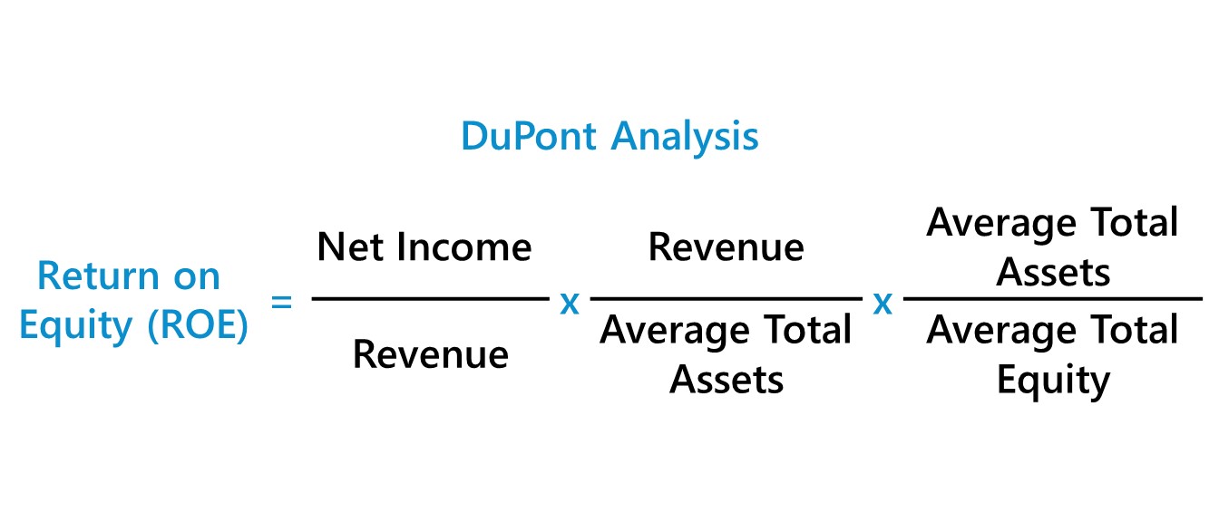
ROE = NI / S * S / TA * TA / E
Equity Multiplier Leverage
TA / E = (E + D) / E = 1 + D/E
Productivity Ratios
average collection period
AR / Net Credit Sales * 365
Total Asset Turnover
Sales / Total Assets
Inventory turnover
COGS / Inv
Days Inventory
365 / Inventory Turnover
Walmart has a days inventory ratio of ~20.
AR Turnover
Sales / AR
Days S/O
AR / S * 365
Economic Value Added
- Capitla = 1000
- wacc = 5%
- capital charge = 50
- ROC = 75/1000 = 7.5%
- EVA = (75 - 50) = 25
- (ROC - wacc) * Capital
Price Per Equity
Interest Coverage Ratio
Dividing a company’s earnings before interest and taxes (EBIT) by its interest expense
TODO: use latex
Compound Leverage Ratio = Interest Burden * Leverage
Earnings management
Earnings management is the practice of using flexibility in accounting rules to improve the apparent profitability of the firm. We will have much to say on this topic in the next chapter on interpreting financial statements. A version of earnings management that became common in the 1990s was the reporting of “pro forma earnings” measures.
Options
The Option Contract
- Call Option:
- gives its holder the right to purchase an asset at a specific price
- Put option:
- gives its holder the right to sell an asset at a specific price
- In the money occurs when exercise would produce positive cash flow
- call option strike price < market price
- put option strike price > market price
Call
- x = 60, P = 3
- Buyer
- Payoff: max ( stock price - x, 0)
- Profit: payoff - premium
Put
- x = 60, P = 3
- Buyer
- Payoff: max ( x - stock price, 0)
- Profit: payoff - premium
American vs. European
American options can be exercised at any time whereas European options can only be exercised on the exercise day.
Types of Options
- Index options
- futures options
- foreign currency options
- interest rate options
Exotic Options
- Asian
- Based on average stock price over a time period
- Payoff is the difference between that average and the strike price
- Based on average stock price over a time period
- Barrier
- depends on the price at expiration as well as if the price crossed a barrier
- knock-out: if the price falls to a certain extent, the option expires worthless
- knock-in: if the price does not fall to a certain extent, the option expires worthless
- Lookback Options
- Depends on the minimum and maximum price of the underlying asset during the life time of the option
- Call option may provide payoff equal to maximum - strike
- Currency-translated options
- asset or exercise prices denominated in a foreign currency
- quanto: fix exchange rate
- digital options
- fixed payoff if a condition is satisfied
Put-Call Parity
- Put-call parity theorem is an equation representing the proper relation between put and call prices
- violation implies arbitrage opportunities
- sell high side, buy low side
- invest cash from sell
Suppose C = 3, P = 3, X = 60, r = 5%, and stock price is 60.
- Sell stock: + 60
- Sell put: + 3
- Buy call -3
- Invest -57.14
- Net: $2.85
In a year or so, the investment becomes $60; You can either buy shares back at 60, your shares get called back at 60 because of the put.
A good “risk-free” asset is CASH.TO
Real example.
Microsoft, 1 year expiry. OTM Call has premium (price) 30.48. Put has a premium of 43.50 with strike of 370. Strike price is 370. risk-free rate is 4%. Stock price is 345.
- 30.48 + 370/1.04 = 345 + 43.5
Straddle
A long straddle is established by buying both a call and a put on a stock, each with the same strike price and expiration date.
A straddle is a bet on volatility. The cost of a straddle is the sum of the call and the put, P + C. Final stock price must depart from X by this cost for the straddle to provide a profit.
Strips and straps are variations of the straddle.
Collars
- Examples
- butterfly
- condor
- limited downside
Futures
Similar to options however with futures and forward contract, there is an obligation to follow through with the agreed-upon transaction.
- Forward contracts call for future delivery at a currently agreed upon price
- Price holds
- Futures contract obliges traders to purchase or sell an asset at an agreed-upon futures price at contract maturity
- Price may fluctuate
- Zero-sum game
- Profit is zero when spot price equals the initial futures price
Future Main Concepts
- Marked to market every day
- Maintenance margin
- Convergence property (futures price and spot price converge at maturity)
Strategies
- Speculators
- Bet whether price will go up or down
- Hedgers
- Protect against price movements
- Long: protect against a higher spot price in the future
- Short: protect against spot prices going down in the future
- Calendar spread
- Long position in a futures contract at one maturity and short in another
Spot-Futures Parity Theorem
- Violation of the parity relationship gives rise to arbitrage opportunities
- Investor holds $1,000 in a mutual fund for S&P500/TSX Index
- Dividends of $20
- The futures contract with delivery in one year trades for $1,010
- Since delivery doesn’t include the delivery of the dividends, the investor can hedge
A perfect hedge should return the risk less rate of return
Arbitrage
- Parity relationship also is called the cost-of-carry relationship
- If the futures price is too high, short the futures and acquire the stock by borrowing the money at the risk-free rate
- If the futures price is too low, go long futures, short the stock and invest the proceeds at the risk-free rate
Spreads
When dividends do not exist, spot–futures parity states that the equilibrium futures price:
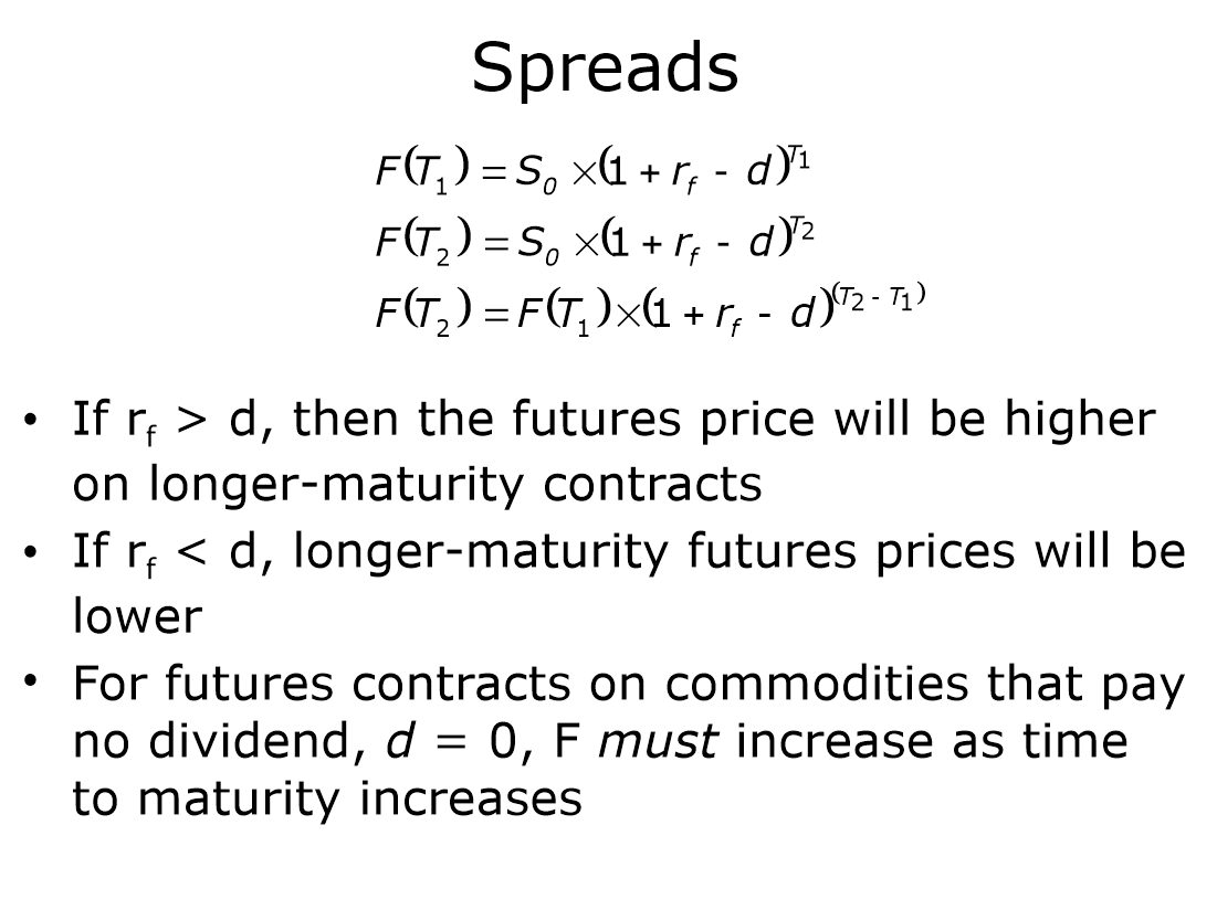
Futures Prices vs. Expected Spot Price
When spot is unchanged:
- Expectations hypothesis
- Future price = the spot price
- Normal backwardation
- Future prices are less and then meet the spot price
- Contango
- future prices are higher and then fall to spot
- Modern portfolio theory